SVM-Based Event Selection for AMANDA 2000-2006

Introduction

A support vector machine (SVM) is a method of classifying data using a machine learning algorithm. SVMs are used widely in high energy physics to solve classification problems very similar to selecting atmospheric neutrinos from misreconstructed cosmic ray muons in AMANDA/IceCube filtered data. The SVM given a number of parameters which differ between signal and background and outputs a single signal/background classification parameter. Some advantages of SVMs include:

• Many data classification parameters are reduced into a single classification parameter, reducing the number of cuts to optimize (ideally, a cut on the SVM parameter would be the only cut necessary).
• SVMs isolate data/background in a higher dimensional space.
• Efficiency should be higher since no hard cuts need to be placed on the data.

Application

Application of an SVM generally follows three steps:

1. Train the SVM on a set of events labeled as signal or background.
2. Test the SVM on data it has not yet seen (to avoid overfitting).
3. Classify the data using the SVM.

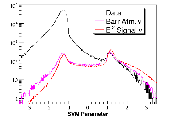
For a point source search, the data at L3 can generally be considered background (1000:1 muon/atm. ν ratio), so the SVM is trained to eliminate data and keep an E^-2 neutrino signal. The advantage of this technique is the background (combination of misreconstructed muons, double muons, cross-talk, etc.) does not need to be explicitly defined. The main disadvantage is any data/MC differences in the distributions of parameters fed to the SVM allow the SVM to eliminate signal from data without penalty. The signal is weighted to favor well reconstructed events.

The data from 2000-2006 and associated Monte Carlo are prepared first by applying light cuts, reducing the data by a factor of 10. This in turn reduces the training/classification time required by the SVM. The cuts are:

• Jkchi(Bayesian) - Jkchi(Pandel) > 23
• Paraboloid Error < 7 deg., σ₁ > 0 && σ₂ > 0
• Flare Sum (TOT_short + B10 + nB10) < 10
• 0 < Phit Smoothness < 0.6

By a process of trial and error, the following parameters are chosen for the SVM classification:

• Jkchi(Bayesian) - Jkchi(Pandel)
• Paraboloid Error
• Phit Smoothness
• Ldir B
• sin(Dec)

The SVM implemented in SVM^light is used. The SVM has three configurable parameters (C, g, j) which must be chosen to optimize the classification. The optimization is done as follows:

• Values of C, g, and j are chosen on a 9 x 9 x 9 grid in powers of log₁₀
• The SVM is trained on 2% of the data (background) and a set of E^-2 neutrino Monte Carlo (signal)
• The resulting SVM model is tested with a new set of data, E^-2 Monte Carlo, and atmospheric neutrino Monte Carlo
• The SVM model is ranked by the passing efficiency of E^-2 Monte Carlo, at a SVM parameter cut level such that Data/Atm. ν < 1.05
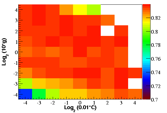
• Near the optimum point, the procedure is repeated on a similar grid in powers of log₂ of each parameter.

The RBF kernel function is used for every configuration. The optimal combination of parameters is found to be (C = 100, g = 0.2, j = 1). The E^-2 efficiency for well-reconstructed events is below for j=1.



A sharp efficiency cutoff exists toward large values of g and j. The SVM is retrained on 5% of the data with the configuration (C = 100, g = 0.2, j = 1) and is used to classify all of the 2000-2006 data and Monte Carlo.


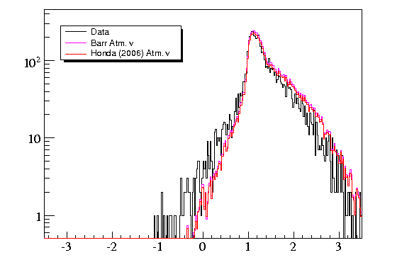
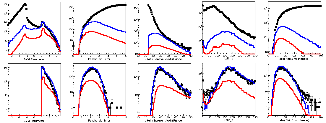
A selection of only events passing the Zeuthen cuts, a high purity atmospheric neutrino sample, indicates high quality atmospheric neutrinos are assigned the proper value (1 is signal-like, -1 is background-like) by the SVM.



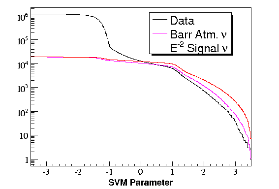
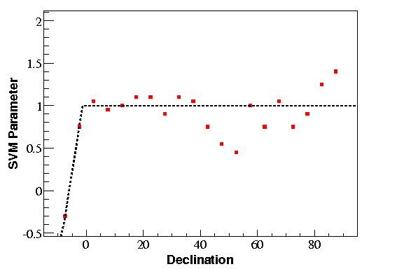
The optimal cut on SVM parameter is determined by MDP optimization. The cut is optimized on a grid of 35 values of SVM parameter and 20 declinations from -7.5^o - 87.5^o using the unbinned search method.

The optimal SVM cut for each declination is shown below, with the chosen cut dotted.



The SVM cut results in 5208 events >10^o, compared with 5409 events using Zeuthen cuts. 87.1% of events in the new sample are present in the Zeuthen sample.

	No Cuts Atm: 61.1% E-2: 66.7% 622K ev >10o
	With SVM Cut Atm: 23.5% E-2: 34.8% 5208 ev >10o

Evaluation

A blind point source analysis is performed on the final event sample. The results are compared to those obtained using a sample chosen with Zeuthen cuts.

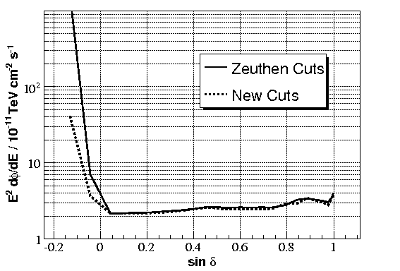
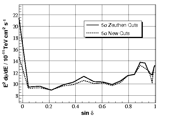
Sensitivity	MDP (P = 0.5)

With the new cuts, average sensitivity and average MDP improves by 3% for positive declinations, with bigger improvements for negative declinations.

Conclusions

The improvement using the SVM is smaller than could be expected. It appears the SVM is selecting events in a very similar fashion to the Zeuthen cuts, so any improvement in sensitivity/MDP is marginal.