DOM-Cal Data Mining

John Kelley, UW Madison, 2 April 2007

0. Overview

DOM-Cal calibration runs record a plethora of data across multiple gain points, including darknoise charge histograms with fit parameters for each DOM. This results in a large quantity of data from which one can determine average DOM parameters, such as:

1. Charge resolution
2. Valley location

and others. These parameters can perhaps be useful in simulation (for defining the "Average DOM") as well as for determining the optimal data-taking parameters for the detector.

1. Charge Resolution vs. Gain

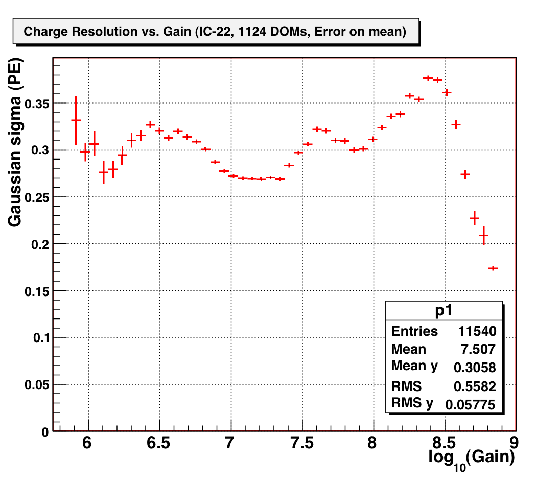
One easily-extracted parameter is the charge resolution, defined as the sigma of the 1-PE Gaussian (in units of PE). This can be plotted as a function of gain for all DOMs (only charge histograms with convergent fits are used):

Figure 1. Charge resolution (Gaussian sigma) as a function of gain, for IC-22 (plus IceTop).

From this plot, a few features are readily observable:

• The optimal gain for best charge resolution (narrow Gaussian) is from 10^7 to 10^7.5 or so.
• There seems to be two populations of DOMs, resulting in the two branches of the distribution at higher gain. No further characterization of these populations is available at this time.

Profile histograms can more clearly show the functional dependence as well as the spread in the distribution at each gain:

Figure 2. Profile histograms of charge resolution vs. gain for IC-22. The left plot shows the error on the mean;
the right, the 1-sigma spread of the population at that point. Keep in mind that the statistics are quite low above 10^8.5.

Once again, the "oscillations" in the profile of the distributions are likely caused by the superposition of the two populations shown more clearly in Figure 1.

2. Valley Location vs. Gain

The "valley" location, defined as the minimum in the charge histogram between the Gaussian and exponential components, is considered by some (at least in the simplest case) as an optimal point for a trigger/discriminator threshold (the situation becomes more complicated in the presence of local coincidence, etc.). The valley location as a function of gain can also be extracted from DOM-Cal data:

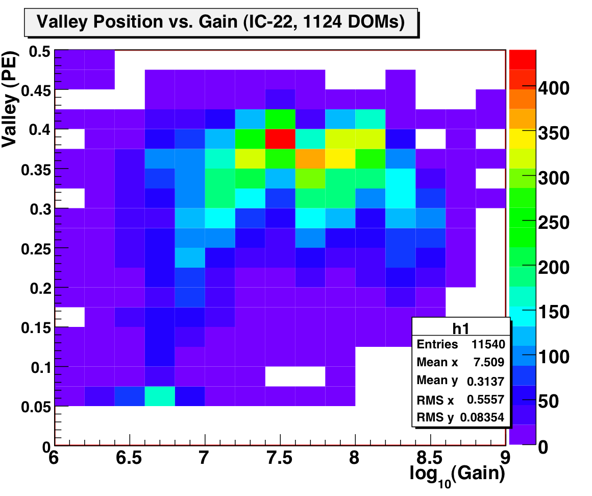
Figure 3. Plot of valley position, in photoelectrons, as a function of gain, for IC-22 (plus IceTop).

Again, this relationship is a bit more clearly visualized with a profile histogram:

Figure 4. Profile plots of valley position as a function of gain. The left plot shows the error on the mean;
the right, the 1-sigma spread of the population at that point. Keep in mind that the statistics are
quite low above 10^8.5 and below 10^6.5.

We anticipate that other DOM parameters can be extracted as well (such as P/V ratio as a function of gain), so stay tuned!