PMT Single Photoelectron Response

John Kelley, UW-Madison, 26 March 2007

0. Executive Summary

Understanding the SPE response of our PMTs is especially important for simulation.
There is a steep low-amplitude exponential component (< ~0.15 PE) of the SPE response which is not noise. There is also possibly a second, less steep exponential component contributing to the "shoulder" of the Gaussian peak in the 0.15-0.4 PE region, although this could be poorly amplified MPE contamination.
The percentage of the distribution below 0.2 PE is highly sensitive to the exponential fit and, according to Chiba measurements, varies from PMT to PMT. This suggests that using an average value obtained from multiple measurements is desirable.
High-statistics averages of the width of the Gaussian portion of the SPE response are available (using DOM-Cal data for IceCube and monitoring data for AMANDA).

1. Introduction

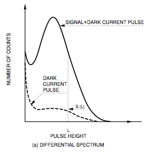
We are familiar with the pulse height / charge distributions for AMANDA OMs and IceCube DOMs — these are often fit by an exponential + Gaussian, with the latter centered at 1 PE (by definition):

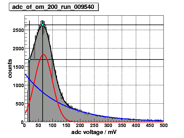
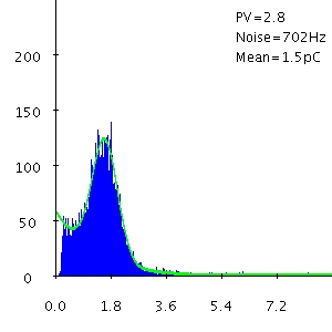
Figure 1: Pulse height / charge distributions, from left to right:
"theoretical" [1], AMANDA OM 200, and IceCube DOM 21-36 ("Glycerol").

The low-amplitude region of the distribution is, according to Hamamatsu, mostly noise [2]. We know, however, that low-amplitude pulses can also arise from imperfect amplification of an SPE from the photocathode — for example, if the electron misses the first dynode.

In an experiment, in practice we eliminate most of the low-amplitude pulses by setting a threshold in the valley of the distributions in figure 1. However, for simulation purposes, we need to decouple the aforementioned effects to understand the response of our PMTs to an SPE, because we know a priori when we simulate this case, and we need an accurate PDF from which to sample our charges / amplitudes.

More precisely, we need the probability distribution function P(charge | SPE), whereas we typically measure P(charge | amplitude > threshold).

2. Measurement of Low-Amplitude SPE Response

It is, however, possible to measure the low-amplitude response by using an external 1 PE light source which triggers the capture window of a DOM, and then by subtracting off the distribution obtained in the same way, but with the light source off. Specifically, we have made the following measurement:

An IceCube DOM in a chest freezer at -25C is illuminated using the mainboard LED. The DOM is set at 1e7 or 5e7 gain.
The LED brightness is set such the DOM sees a single PE approximately 2% of the time.
The LED trigger also triggers the ATWD capture window. The peak of the waveform (regardless of whether an SPE is present) is integrated to obtain the charge, and the timing of the peak position is recorded. A large, fixed number of triggers are recorded.
The same procedure is followed with the LED power off but still triggering the capture window at the same fixed rate.

Using ATWD channel 0 at a high sampling speed allows excellent charge resolution. We find the following charge distribution at 1e7 gain for LED on/off states:

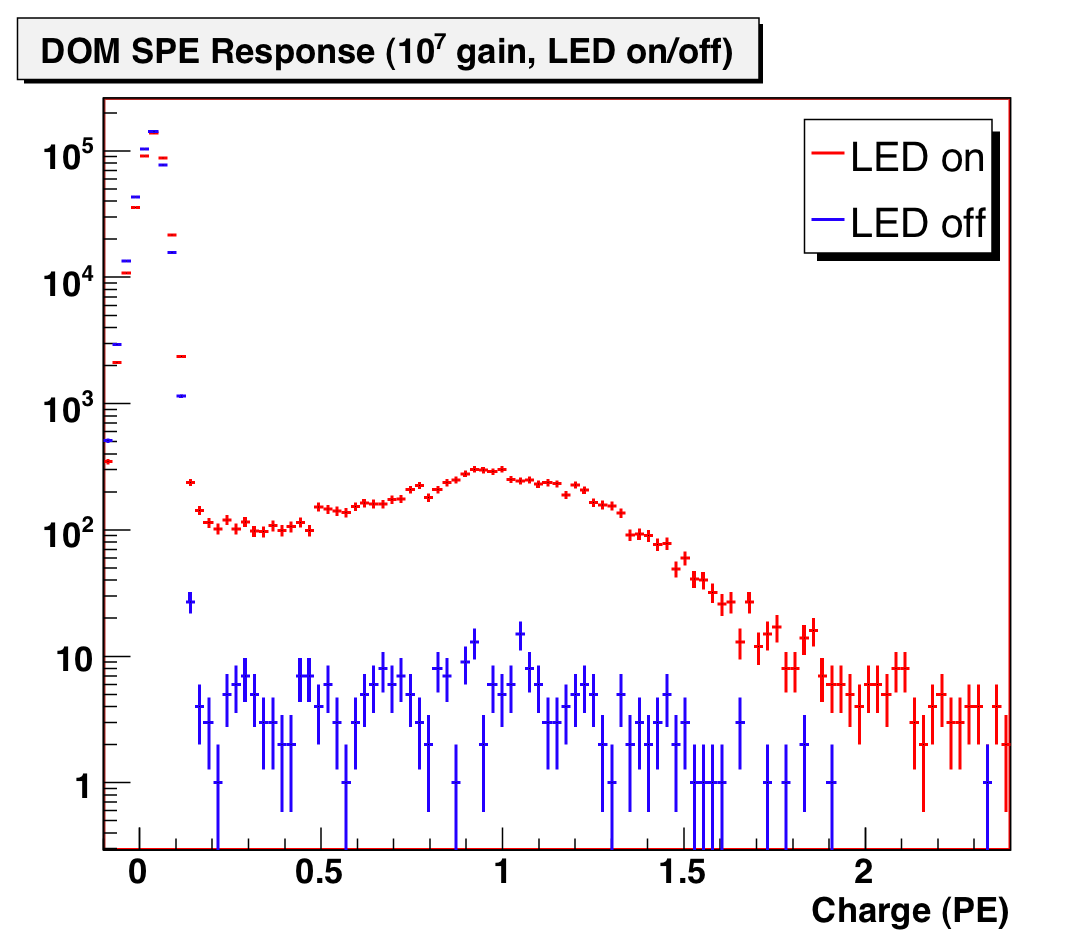
Figure 2: DOM response to mainboard LED (both on and off states) at 1e7 gain, -25C.

At 10^7, non-random noise in the waveform (due mostly to imperfect baseline slope calibration) dominates below 0.15 PE, so we are unable to fit this region. However, the exponential component fit from Q>0.15 PE is not very steep. Subtracting one from the other, we find the follow as the SPE response above 0.15 PE:

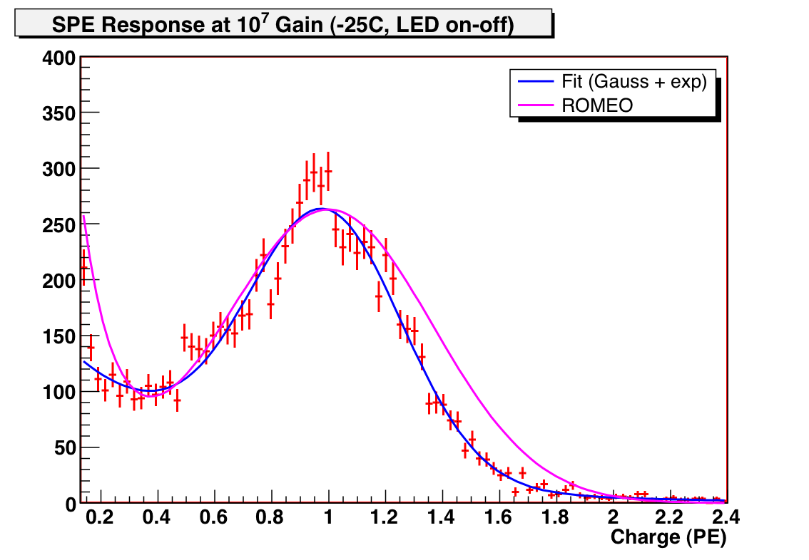
Figure 3: SPE Response of DOM above 0.15 PE, with ROMEO model overlaid.
Exponential component is not very steep in the 0.15-0.5 PE region,
but there is a hint of steeper component in last data point.

With the fit above, the fraction of pulses below 0.20 is ~11%, compared to 23% in the ROMEO model.

To understand the low-amplitude behavior, we increase the gain to 5x10^7. This allows reliable charge determination for pulses with Q < 0.10 PE:

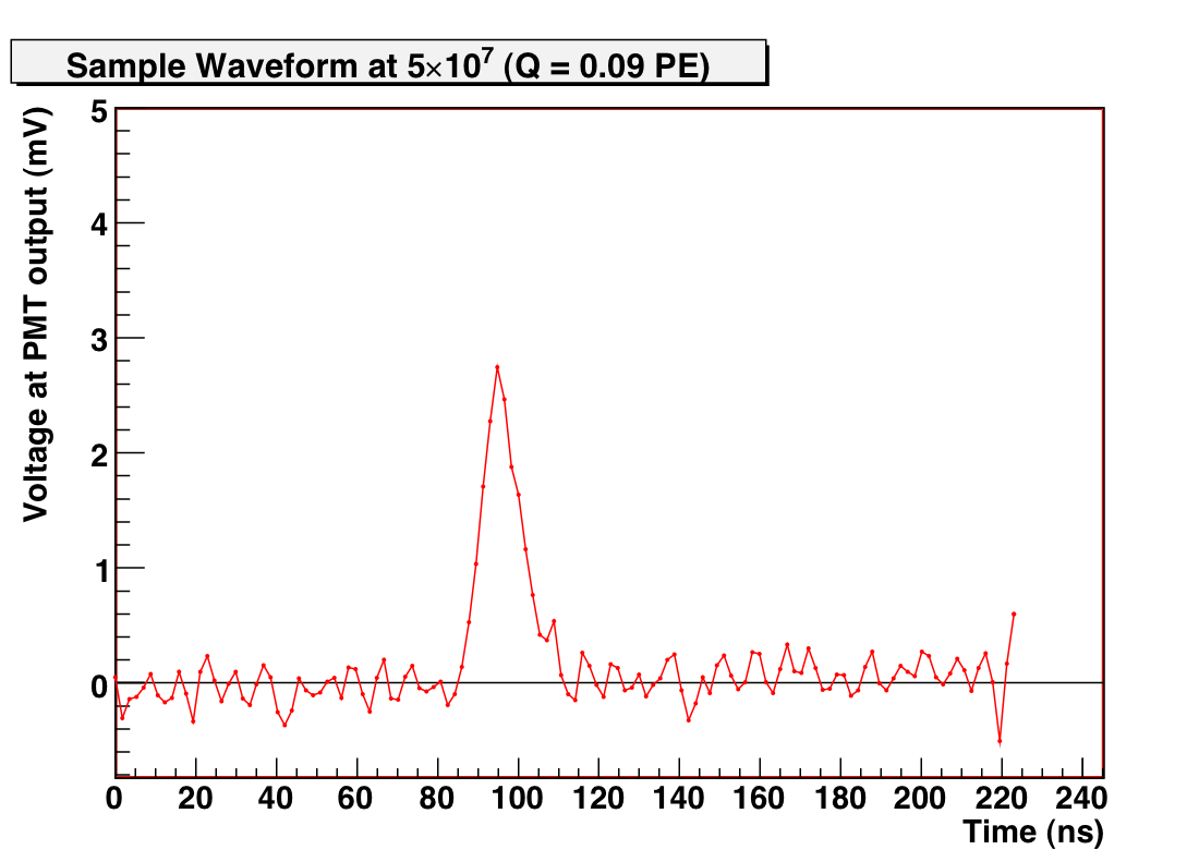
Figure 4: Sample waveform of small charge (Q = 0.09 PE) at 5e7 gain (calibrated ATWD ch0).

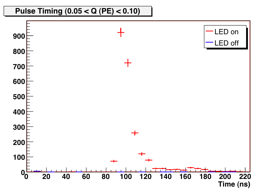
We find that there is a steep exponential component below Q = 0.15 PE. This is demonstrably part of the SPE response, and not noise, by examining the timing information of these low-amplitude pulses — we find that they occur when the SPE response is expected:

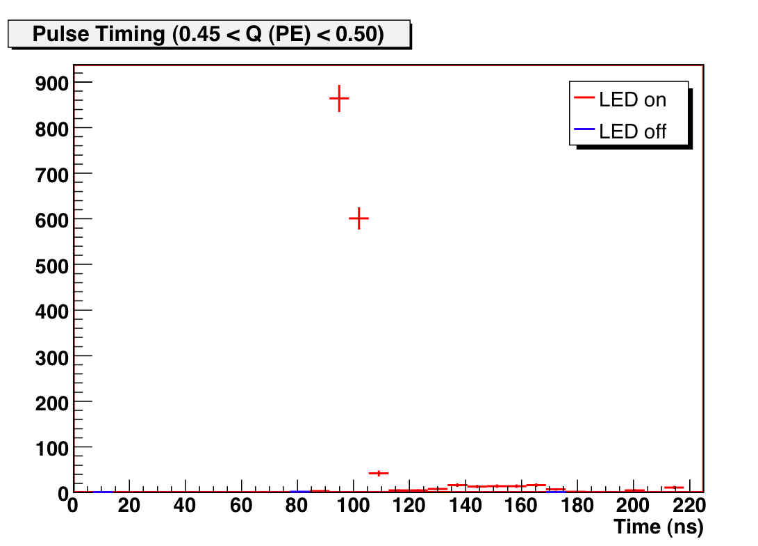Figure 5: Timing information at 5e7 gain of pulses of various charge.
~100ns is the timing expected for a fully amplified SPE.

The total response is fit best by a Gaussian plus two exponentials:

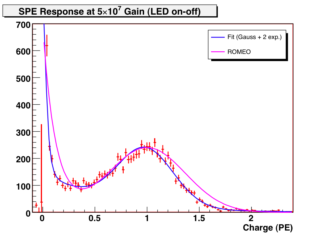
Figure 6: DOM SPE response at 5e7 gain, with ROMEO model overlaid (2% SPE occupancy).

With this fit, the fraction of the response below 0.2 PE is 22%, compared to 23% in the ROMEO model.

UPDATE: At higher SPE occupancy (25%), the flatter exponential component has been significantly enhanced due to MPE contamination:

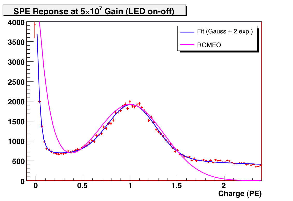
Figure 7: DOM SPE response at 5e7 gain, with ROMEO model overlaid (25% SPE occupancy).

This suggests that perhaps the low-amplitude "shoulder" of the Gaussian, which dominates between 0.15 and 0.4 PE, could still be MPE contamination (poorly amplified!), but this is unconfirmed.

3. Width of Gaussian Peak

The width of the Gaussian portion of the SPE response is easy to measure for large ensembles of OMs and DOMs. For AMANDA OMs, we have the online ADC fits from the monitoring pages. For IceCube DOMs, we have fits to the charge histograms over multiple voltages for every DOM, via the DOM-Cal result XML files.

For all good AMANDA OMs with reasonable fits (N=585), using monitoring data from run 9529 in 2005:

AMANDA average sigma/mu = 0.46 +/- 0.10 PE

For all good IceCube and IceTop DOMs with reasonable fits at 10^7 voltage (N=497), using DOM-Cal run from 8/21/2006:

IceCube average sigma/mu = 0.29 +/- 0.09 PE

References:

"Photomultiplier Tubes: Basics and Operation", Hamamatsu Corporation, p. 141.
"[Photomultiplier Tube] Construction and Operating Characteristics", Hamamatsu Corporation, p.12.

Back to home page