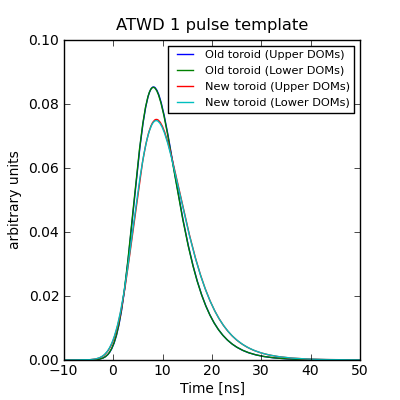
Pulse shapes in low-gain ATWD channels
Introduction
The mean SPE pulse shapes in the FADC and ATWD channel 0 have already been characterized from flasher data in a study by Chris Wendt. However, the frequency responses of the 3 ATWD channels are not identical, and the pulse shapes in the lower-gain channels have to be characterized separately in order to properly handle high-amplitude waveforms in the ATWD.
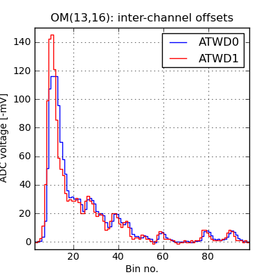
An example of the effect of the different frequency responses of ATWD channels 0 and 1. The response from channel 1 leads channel 0 by approximately the width of the one bin (3.33 ns).
Method
Since the arrival time of the PMT pulse is implicit in the parameterization of the pulse shape for ATWD channel 0, we can use it to bootstrap templates for the other ATWD channels that have the same definition of the arrival time. We do this by first noting that we expect the trace in the ATWD to be a convolution of some true input signal with the ATWD pulse shape for each channel:
where \(a_0\) and \(a_1\) are the measured traces in ATWD channels 0 and 1, \(V\) is the input signal and \(f_0\) and \(f_1\) are the pulse shapes in each channel. Given waveforms measured simulaneously by both channels 0 and 1 and a parameterization of the channel 0 pulse shape, we can solve for an approximate representation of the unknown ATWD channel 1 pulse shape. Since convolution is the same as multiplication in frequency space, we can take the Fourier transform of all these quantities in order to more easily manipulate them. Then:
In other words, we find the “difference kernel” that maps channel 0 onto channel 1, then convolve this with the channel 0 pulse shape to obtain the channel 1 pulse shape.
Implementation
This method would of course only work perfectly for either infinitely long waveforms or infintessimal time binning. With a large enough number of waveforms, though, it can be made to produce acceptable results with our short waveforms.
Channel 1
Selection
I began by selecting events from Run 117660 (an unfiltered IC86 test run from 2011-01-29) where at least ATWD channel 1 was present in the readout. I calibrated all ATWD channels separately using WaveCalibrator. For the channel 1 fits, I selected relatively low-amplitude waveforms, where channel 0 remained unsaturated and the peak voltage in all channels was between 7 and 20 mV.
Deconvolution
For each pair of ATWD channel 0/1 waveforms, I extracted an approximate representation of \(\hat{f_1}(k)\) using an FFT:
def deconvolute(wf1, wf2):
        # evaluate pulse template at right-hand edge
        t = wf1.bin_width*numpy.arange(1, 129, dtype=float)

        # f1 is the impulse response responsible for a1
        f1 = wavereform.spe_atwd_new(t) # arbitrary normalization
        a1 = numpy.array(wf1.waveform)/icetray.I3Units.mV
        a2 = numpy.array(wf2.waveform)/icetray.I3Units.mV
        # fourier-transform all the inputs
        a1_hat = numpy.fft.fft(a1)
        a2_hat = numpy.fft.fft(a2)
        f1_hat = numpy.fft.fft(f1)
        # extract approximate difference kernel, then convolve with ch0 impulse
        f2_hat = (a2_hat/a1_hat)*f1_hat

        # extract the approximate impulse response that made a2
        f2 = numpy.sqrt(a1_hat.size)*(numpy.fft.ifft(f2_hat).real)

        return f2
An example of the deconvolution is shown below.
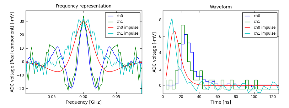
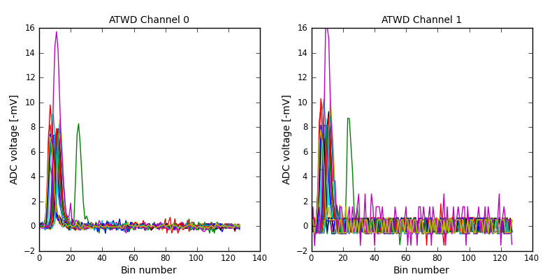
The first 20 pairs of waveforms used to extract the ATWD 1 pulse shape.
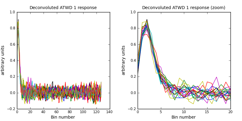
Individual deconvolutions of the channel 1 response from the first 20 pairs of waveforms. These are later averaged and fit to a function.
Fitting
Next, I fit a function with the same form as the other pulse templates,
to the average of the approximate \(\hat{f_1}(k)\):
def pulse_template(time, args):
        c, x0, b1, b2 = args
        t = time - 11.5 # shift for causality
        func = c*(numpy.exp(-(t - x0)/b1) + numpy.exp((t - x0)/b2))**-8
        return func

def fit_response_fft(waveforms, plot=True):
        # extract approximations of the channel 1 pulse shape
        arr=numpy.vstack([deconvolute(*wf) for wf in waveforms])

        # evaluate template function at right-hand edge
        t = waveforms[0][0].bin_width*numpy.arange(1, 129, dtype=float)

        # new-toroid ATWD shape with an arbitrary normalization
        # that happens to match the what we're fitting
        c = 1; x0 = -4.24 - 5; b1 = 5.5; b2 = 42.;
        init = [c, x0, b1, b2]

        from scipy.optimize import fmin
        from scipy.integrate import quad

        def chi2(args, t, y):
                chi = ((pulse_template(t,args)-y)**2).sum()
                return chi

        # Since fourier transforms are periodic, wrap it around.
        deconvoluted = numpy.concatenate((arr[64:], arr[:64]))
        t = numpy.concatenate((t[64:]-t[-1], t[:64]))

        optimized = fmin(chi2, init, args=(t, deconvoluted), maxfun=100000, xtol=1e-6, ftol=1e-6)

        # normalize it
        norm = quad(pulse_template, -50, 500, args=optimized)[0]

        deconvoluted /= norm
        optimized[0] /= norm

        if plot:
                pylab.figure()
                pylab.plot(t, deconvoluted, ls='steps', label='Average ATWD 1 response')
                pylab.plot(t, deconvoluted.transpose(), ls='steps')

                t = numpy.linspace(-50, 500, 1000)
                pylab.plot(t, pulse_template(t, optimized), label='Fit')
                pylab.plot(t, wavereform.spe_atwd1_new(t), label='ATWD 0 pulse template')
                pylab.legend()
                pylab.xlabel('Time [ns]')
                pylab.ylabel('arbitrary units')

        return optimized
The result of the fit to the new-toroid DOMs on String 58 is shown below.
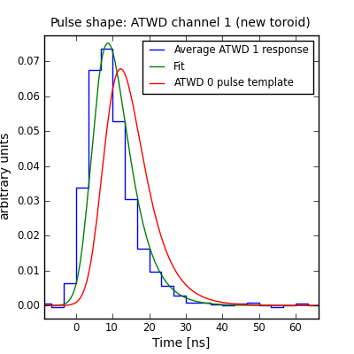
A fit to the ATWD channel 1 pulse shape, as extracted from joint channel 0/1 readouts.
Channel 2
Selection
The procedure for Channel 2 is the same as for Channel 1, except with notably smaller statistics. For these fits, I selected all waveforms from Run 117660 where Channel 1 measured a peak voltage above 100 mV (roughly 10 counts in Channel 2), but did not saturate. This yielded 315 waveform pairs in old-toroid DOMs and 1443 in new-toroid DOMs.
Deconvolution
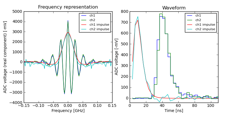
Again, the procedure is similar, with the exception that the Channel 1 pulse shape is the one bootstrapped from Channel 0 rather than fit directly from single-PE waveforms. An example deconvolution is shown below.
Results
The fit parameters are summarized in the following table:
| Model | c | x0 | b1 | b2 |
|---|---|---|---|---|
| Old toroid ATWD 0 (Chris Wendt) | 1.16 | -8.93 | 4.70 | 39.00 |
| Old toroid ATWD 1 | 2.07 | -10.96 | 4.86 | 30.75 |
| Old toroid ATWD 2 | 1.36 | -9.69 | 3.50 | 30.97 |
| New toroid ATWD 0 (Chris Wendt) | 1.20 | -9.24 | 5.50 | 42.00 |
| New toroid ATWD 1 | 1.66 | -11.70 | 5.47 | 36.22 |
| New toroid ATWD 2 | 0.71 | -10.59 | 3.48 | 42.11 |
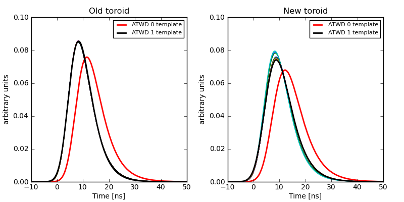
Comparison of fits to the ATWD channel 1 pulse shape with a fit to the ATWD channel 0 pulse shape by Chris Wendt. The results of fits to random groups of 1000 waveforms are shown in thin lines; for the old-toroid DOMs these are entirely hidden by the overall fit line.
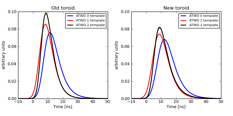
Comparison of fits to the ATWD channel 2 pulse shape with the channels 0 and 1 pulse hapes.
Verification
If we have the correct pulse shapes, then we should be able to unfold essentially the same pulses from either ATWD channel 0 or 1 and predict the trace in one digitizer from the other. An example is shown below.
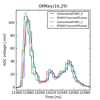
An example of a pulse series unfolded from ATWD channel 0, then refolded with the pulse shape for each channel. When the different pulse shapes are taken into account, the refolded trace matches the measured trace in each digitizer almost equally well.
Refolding
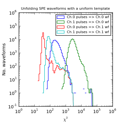
This can be done a little more systematically using a large sample of single-PE waveforms where the DOM transmitted both ATWD channels 0 and 1 to the surface (66k waveforms from Run 117661). First, I unfolded pulses from each waveform separately using Wavedeform, then calculated a \(\chi^2\) between each waveform and pulse series using Wavereform. Because the unfolding doesn’t know about the different pulse shapes, the aggreement between the refolded pulse series and the waveform changes by a large amount depending on which digitizer was used:
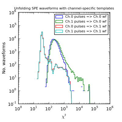
Next, I gave Wavedeform the ability to use different pulse shapes for each ATWD channel. When this is done, the two digitizer channels are handled much more constently. Since channel 0 is discretized roughly 8 times more finely than channel 1, the \(\chi^2\) distribution for channel 1 shows that channel 0 is just as good at predicting what channel 0 measured as channel 1 itself. For the same reason, the \(\chi^2\) for channel 0 is worse when the pulses are unfolded from channel 1, but not significantly so in most cases.
Normalization
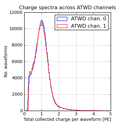
The pulse templates are normalized such that they integrate to 1. This produces charge spectra with a peak at 1 PE in both ATWD channel 0 and 1. This is difficult to check for channel 2, as a PE pulse is typically less than 1 count high in that channel.
Variability between DOMs
The pulse template parameters provided here are derived from an average over many DOMs, and it is possible that the pulse template depends on factors other than the toroid type. For example, the DOMs at the top of the array have a systematically lower operating temperature than those at the bottom. This can be (roughly) checked by doing the fit separately on the upper and lower halves of the array and comparing the results. The maximum difference is less than 1%, at the peak of the new-toroid template.
