Predicting observable distributions
To estimate the sensitivity of proposed Gen2 detector layouts, event selections, and reconstruction techniques to various model tests, we need to be able to predict the mean event rate in bins in some observable space, and use the Asimov method outlined above to derive significance contours in the space of the model parameters. The most general and precise way to do this is to treat the conversion from particle fluxes to event rates as a Monte Carlo integral, simulating neutrino and penetrating atmospheric muon events and filling the observables for each simulated event into an \(n\)-dimensional histogram with weights calculated from the true properties under the hypothesis in question, e.g. atmospheric neutrinos plus some amount of quasi-diffuse astrophysical flux. This approach has two disadvantages, however:
1. It only works well when one has enough simulated events that every bin in the observable space is sufficiently populated that the statistical error on the mean is much smaller than the expected Poisson fluctuations. In particular, no bin must be completely empty. This is already difficult to acheive for the existing detector, and will only be worse for a multitude of proposed upgrade designs.
2. It hides the influence of key performance numbers on the total sensitivity, e.g. it is not especially straightforward to gauge how a 2x improvement in angular resolution above 10 TeV would influence the sensitivity to steady point sources.
We can skirt both of these issues at the cost of some loss in precision by factorizing the conversion into its component parts. The decomposition is slightly different for each detection channel.
Throughgoing muon tracks
Muon production efficiency
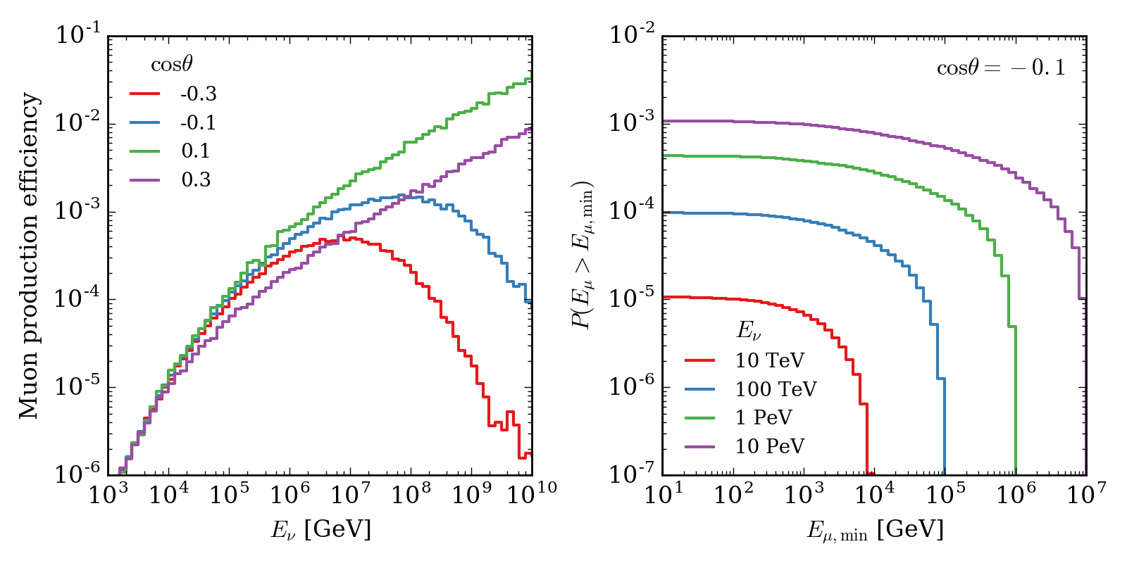
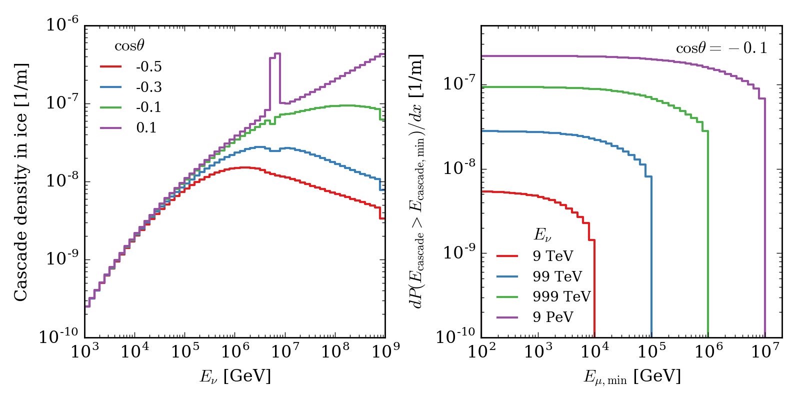
To convert a flux of neutrinos to a flux of muons at the detector, we need to know the probability that a neutrino of a given energy \(E_{\nu}\) and zenith angle \(\theta\) will produce a muon that reaches the detector border with energy \(E_{\mu}\). We obtain this probability by simulating muon neutrinos and antineutrinos with NeutrinoGenerator and propgate any muons that may result to the surface of a 1000x500 meter cylinder with PROPOSAL. We fill the energy of the neutrino, its zenith angle, and the energy of the muon at the detector border into a 3D histogram with a weight given by
The final production efficiency is given by the entries in this histogram, divided by the width of the bins in neutrino energy and solid angle. Experienced NuGen users will recognize this as the usual neutrino effective area, divided by the injection area to make it unitless, and separated into bins in true muon energy at the detector border.
The left panel of the figure below shows the muon production efficiency at several zenith angles, averaged over neutrinos and antineutrinos and integrated over all muon energies greater than zero. The right panel shows the cumulative distribution of muon energies in several neutrino energy bins at a single zenith angle. These are the elements of a transfer matrix that converts neutrino fluxes into detectable muon fluxes.
(Source code, png, hires.png, pdf)
This formulation approximates the detector volume as a point, and is only valid as long as the scale size of the detector volume is much smaller than a) the interaction length of neutrinos in the ice sheet (so that instrumented region does not shadow itself in neutrinos), and b) the curvature radius of the earth (so that the average overburden as a function of zenith angle is nearly the same for different detector sizes).
Geometric area
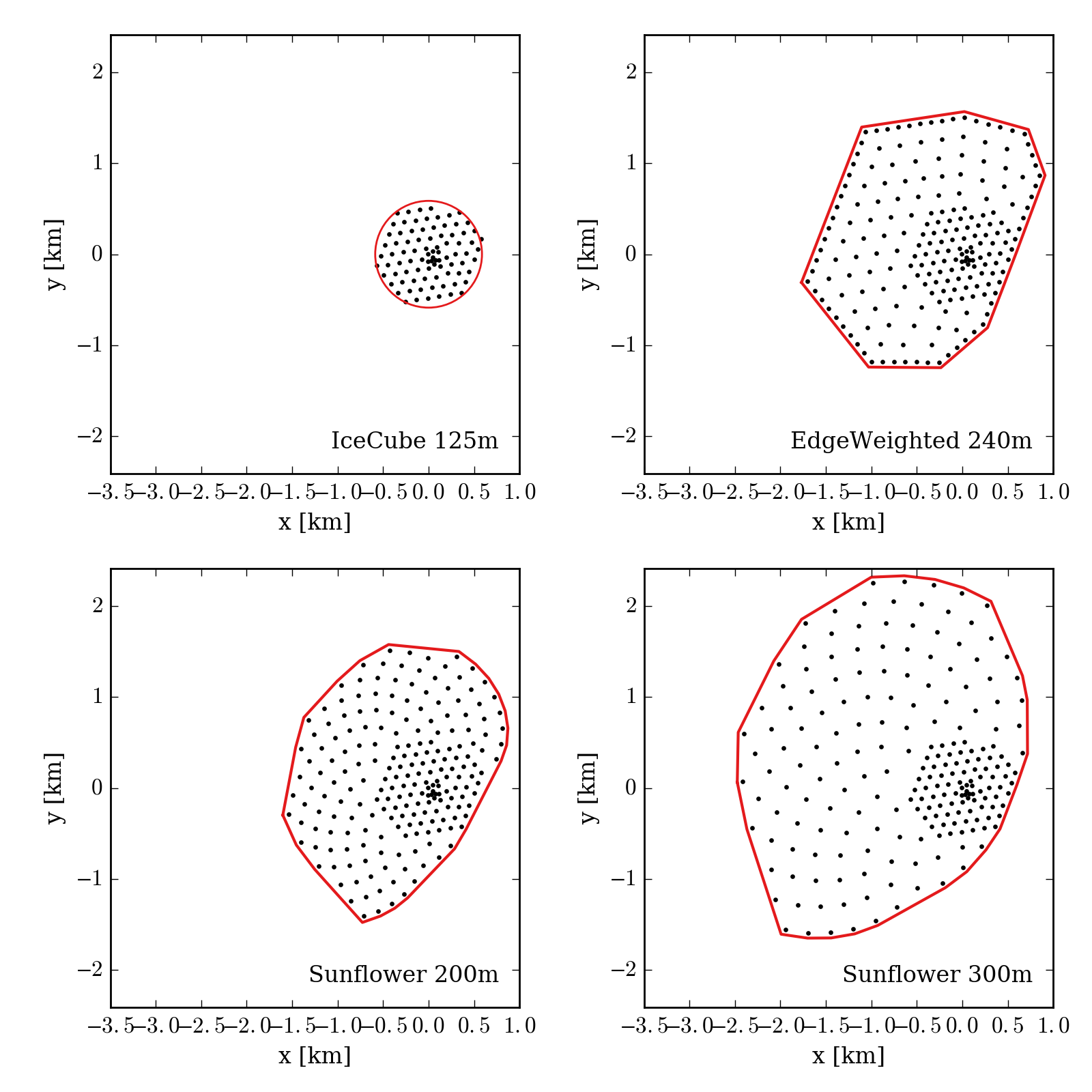
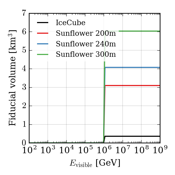
Now we need to take the geometry of the detector into account to convert the dimensionless muon production efficiency into an effective area for each proposed detector configuration. For each detector, we define a fiducial surface; muons that cross this surface should be detectable. The figure below shows the positions of the strings in a few detector configurations as black dots and the outline of the fiducial surface as a red line. The fiducial surface for IceCube is a cylinder with a size chosen in the muon effective area calculation for the Aachen multi-year diffuse analysis, while the fiducial surface for the Gen2 geometries is the convex hull of the strings, with each face moved outward by 60 m.
(Source code, png, hires.png, pdf)
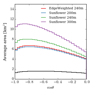
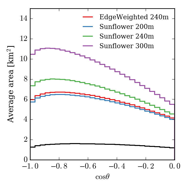
The figure below shows the area of several geometries averaged over a zenith band. The fiducial area of IceCube is given in black for comparison.
(Source code, png, hires.png, pdf)

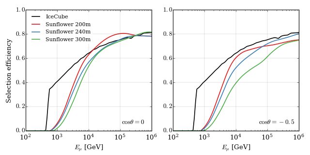
Muon selection efficiency
Once muons have reached the detector, the muon events have to pass the event selection. We parameterize the selection efficiency as a function of zenith angle and muon energy at the detector border as shown in the figure below.
(Source code, png, hires.png, pdf)

The selection efficiency is defined as the ratio of the muon effective area to the geometric area, which can be obtained easily from MuonGun simulation.
Muon energy resolution
TODO: describe
Muon angular resolution
The distribution of the opening angle between the true muon direction and the reconstructed direction is parameterized as a function of muon energy as shown in the figure below. The opening angle between neutrino and muon (significant below 1 TeV) is neglected.
Starting events
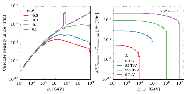
Energy deposition density
(Source code, png, hires.png, pdf)

(Source code, png, hires.png, pdf)

TODO