Photospline

Detector response to a high-energy physics process is often estimated by Monte Carlo simulation. For purposes of data analysis, the results of this simulation are typically stored in large multi-dimensional histograms, which can quickly become unwieldy in terms of size or numerically problematic due to unfilled bins or interpolation artifacts. Photospline is a library that uses the penalized spline technique to efficiently compute, store, and evaluate B-spline representations of such tables.

Fitting tutorial

A basic fitting script starts with a few imports:

import numpy
from icecube.photospline import spglam as glam
from icecube.photospline import splinefitstable
from icecube.photospline.glam.glam import grideval
from icecube.photospline.glam.bspline import bspline

Some of these are strictly required.

• numpy - We need this in order to pass n-dimensional arrays around
• glam - We will use the sparse-matrix implementation of the least-squares fit. Replace this line with from icecube.photospline.glam import glam in order to use the inefficient (but readable) Python reference implementation.
• splinefitstable - We will use icecube.photospline.splinefitstable.write() to store the fit results in a FITS file.

We will also need some extra functions in order to visualize the result.

• grideval - We will use this function to evaluate the spline surface on a coordinate grid.
• bspline - We will also plot the individual basis functions to get a better idea of how the spline surface is constructed.

For this example, we will make up some random, one-dimensional data drawn from a cosine overlaid on a polynomial:

numpts = 500
x1 = numpy.sort(numpy.random.uniform(-4,25,size=numpts))
z = numpy.random.poisson(numpy.cos(x1)**2 + (x1-3.0)**2 + 10)

We can improve the quality of the fit by giving less weight to data points that are likely to be distorted by statistical fluctuations. Here we’ll use a minimum weight of 1, and weight the high-occupancy points up:

w = 1. + z

Now we need to choose a set of B-spline basis functions. We will use a grid of order-2 B-splines that extend beyond the the data points, relying on the regularization term for extrapolation:

order = 2
knots = [numpy.linspace(-8,35,30)]
smooth = 3.14159e3

This generalizes easily to multi-dimensional data; we would simply add an extra entry to knots for each extra dimension.

To actually run the fit, we call icecube.photospline.spglam.fit()

>>> result = glam.fit(z,w,[x1],knots,order,smooth)
Calculating penalty matrix...
Calculating spline basis...
Reticulating splines...
        Convolving bases...
                Convolving dimension 0
        Flattening residuals matrix...
Transforming fit array...
Computing least square solution...
Analyze[27]: 0.000049 s
Factorize[27]: 0.000027 s
Solve[27]: 0.000022 s
Done: cleaning up

Now we can save the fit result for later use with ndsplineeval() or icecube.photospline.glam.glam.grideval()

splinefitstable.write(result, 'splinefit-1d.fits')

To see the result, we can plot it with matplotlib:

import pylab
# Plot individual basis splines
xfine = numpy.linspace(knots[0][0], knots[0][-1], 10001)
splines = [numpy.array([bspline(knots[0], x, n, order) for x in xfine]) for n in range(0,len(knots[0])-2-1)]
for c, n in colorize(range(len(splines))):
        pylab.plot(xfine, result.coefficients[n]*splines[n], color=c)
# Plot the spline surface (sum of all the basis functions)
pylab.plot(xfine, glam.grideval(result, [xfine]), label='Spline fit', color='k')
pylab.legend(loc='upper left')
pylab.show()

The result is shown below:

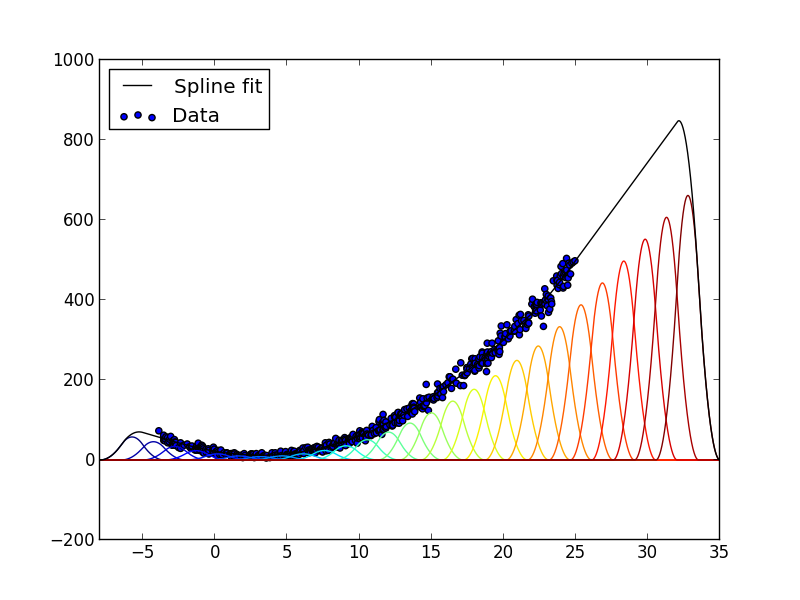
Example 1-dimensional spline fit. The spline surface (black line) is the sum of basis functions (colored lines) weighted with coefficients determined by a linear least-squares fit to the data (blue dots). In the region to the right where there are no data, the order-2 penalty term produces a straight line.

Python library reference

The interface to the fitting library is entirely in Python, using Numpy arrays to as containers for the data, spline coefficients, knot vectors, etc. The spline coefficients determined in the fit are stored in FITS files that can be loaded and evaluated using the bundled C library.

Note

The reference Python fitting implementation icecube.photospline.glam.glam.fit() uses dense matrix operations from numpy, and can become extremely memory-hungry in large numbers of dimensions.

The C implementation icecube.photospline.spglam.fit() implements the same functions as the Python version, but uses sparse matrix operations from SuiteSparse. This is both orders of magnitude faster and uses 100x less memory for typical problems. You should use spglam for large-scale fitting and fall back to glam if necessary for debugging.

icecube.photospline.glam.glam.fit(z, w, coords, knots, order, smooth, periods=None, penalties={2: None}, bases=None, iterations=1, monodim=None, dump=False)

Fit gridded data to a B-spline surface.

Parameters:

• z – An ndarray containing the data to be fit
• w – An ndarray of weights for each data point. If you don’t want to weight the data points differently from each other, use uniform weights (e.g. numpy.ones(z.shape)).
• coords – A list of coordinate axes giving the location of the data points in each dimension. Each coordinate axis must have the same length as the corresponding dimension in z.
• knots – A sequence of knot vectors, each giving the location of the B-spline knots in the cooresponding dimension.
• order – The order of the B-spline surface. If this is a single integer the order will be the same for all dimensions; you can also pass a list of integers to specify the order to use in each dimension individually.
• smooth – The global smoothing parameter . This will be used only if no dimension-specific smoothing is specified in penalties.
• periods – A list of floats, each giving the periodicity of the corresponding dimension. If the periodicity is nonzero, the fit will use a periodic B-spline basis in that dimension where the ends are identical by construction. This functionality is only implemented in glam; spglam will silently ignore the periodicity of the basis.
• penalties – A dictionary giving the penalty term to apply along each dimension. Each key-value pair specifies an order of penalty and the coefficient of that penalty order in each dimension. For example, to apply second-order penalties in the first three dimensions and a third-order penalty in the fourth (all with ), you would pass {2:[1,1,1,0], 3:[0,0,0,1]}. If the coefficient list is None (as it is by default), the specified by smooth will be used for all dimensions.
• monodim –

  If set to a non-negative integer, the spline surface will be forced to be monotonic along the corresponding dimension.

  Note

  This involves solving a non-negative least squares problem, and is thus significantly slower than an unconstrained fit.

Returns:

SplineTable - the fit result

icecube.photospline.spglam.fit(z, w, coords, knots, order, smooth=1, periods=None, penalties=None, monodim=None)

A drop-in replacement for icecube.photospline.glam.glam.fit().

icecube.photospline.splinefitstable.write(table, path)

Write a SplineTable to disk as a FITS file.

Parameters:

• table – the SplineTable to be written
• path – where to save the FITS file.

Warning

pyfits will fail to write the file if it already exists.

icecube.photospline.splinefitstable.read(path)

Read a SplineTable from a FITS file on disk

Parameters:path – the filesystem path to read from Returns:SplineTable - the spline surface stored in the given file

icecube.photospline.glam.glam.grideval(table, coords, bases=None)

Evaluate a spline surface on a coordinate grid

Parameters:

• table – The spline surface to be evaluated
• coords – A sequence of coordinate axes, one for each dimension in the spline table.

Returns:

an array of values, one for point in the tensor product of the supplied axes

>>> spline.coefficients.ndim
2
>>> grideval(spline, [[0, 0.5, 1.0], [0.5, 1.0]])
array([[ 1482.110672  ,  4529.49084473],
       [ 1517.94447213,  4130.34708567],
       [ 1506.64602055,  3425.31209966]])

icecube.photospline.spglam.grideval(table, coords)

A drop-in replacement for icecube.photospline.glam.glam.grideval().

Note

The bases argument is not supported in this version.

icecube.photospline.glam.glam.bspline(knots, x, i, n)

Evaluate the ith nth-order B-spline basis function at x.

Parameters:

• knots – a sequence of knot positions
• x – the position at which to evaluate the spline
• i – the index of the basis function
• n – the order of the spline

Returns:

float - the value of the spline at x

C library reference

The photospline C library contains a collection of functions for efficiently evaluating the tensor-product B-spline surfaces produced by :py:func`icecube.photospline.spglam.fit` and written to disk as FITS files by icecube.photospline.splinefitstable.write().

Spline table I/O and manipulation

struct splinetable

A data structure that holds the coefficients, knot grids, and associated metadata needed to evaluate a spline surface:

struct splinetable {
        int ndim;
        int *order;
        double **knots;
        long *nknots;
        double **extents;
        double *periods;
        float *coefficients;
        long *naxes;
        unsigned long *strides;
        int naux;
        char ***aux;
};

int readsplinefitstable(const char *path, struct splinetable *table)

Read a spline table from a FITS file on disk.

Parameters:

• path – the filesystem path to read from
• splinetable – a pointer to a pre-allocated splinetable

Returns:

0 upon success

int readsplinefitstable_mem(struct splinetable_buffer *buffer, struct splinetable *table)

Read a spline table from a FITS file in memory.

Parameters:

• buffer – The memory buffer to read from. data must point to the beginning of the memory area where the FITS file is stored, and size should give its size. mem_alloc and mem_realloc must be set to valid addresses, but will not be called.

Example:

struct splinetable table;
struct splinetable_buffer buf;

readsplinefitstable("foo.fits", &table);
buf.mem_alloc = &malloc;
buf.mem_realloc = &realloc;
writesplinefitstable_mem(&buf, &table);
splinetable_free(&table);

readsplinefitstable_mem(&buf, &table);
free(buf.data);
/* do stuff with table */
splinetable_free(&table);

int writesplinefitstable(const char *path, const struct splinetable *table)

Write a spline table to a FITS file on disk.

int writesplinefitstable_mem(struct splinetable_buffer *buffer, const struct splinetable *table)

Write a spline table to a FITS file in memory.

Parameters:

• buffer – the memory buffer to write to. Memory will be allocated internally via mem_alloc and mem_realloc, which should point to malloc() and realloc() or functional equivalents.

Example:

struct splinetable table;
struct splinetable_buffer buf;

readsplinefitstable("foo.fits", &table);
buf.mem_alloc = &malloc;
buf.mem_realloc = &realloc;
writesplinefitstable_mem(&buf, &table);
splinetable_free(&table);
/* do stuff with buf */
free(buf.data);

char * splinetable_get_key(struct splinetable *table, const char *key)

Get a pointer to the raw string representation of an auxiliary field stored in the FITS header.

Parameters:

• key – A null-terminated string containing the key.

Returns:

A pointer to the beginning of the value string, or NULL if the key doesn’t exist.

int splinetable_read_key(struct splinetable *table, splinetable_dtype type, const char *key, void *result)

Parse and store the value of an auxiliary field stored in the FITS header.

Parameters:

• type – The type of value stored.
• key – A null-terminated string containing the key.
• result – Where to store the result

Returns:

0 upon success

splinetable_dtype

Types that can be parsed by splinetable_read_key():

typedef enum {
        SPLINETABLE_INT,
        SPLINETABLE_DOUBLE
} splinetable_dtype;

void splinetable_free(struct splinetable *table)

Free memory allocated by :c:function:`readsplinefitstable`.

Spline evaluation

int tablesearchcenters(const struct splinetable *table, const double *x, int *centers)

Find the index of the order-0 spline in each dimension that has support at the corresponding coordinate.

Parameters:

• x – an array of coordinates, one for each dimension
• centers – the array where the index corresponding to each coordinate will be stored.

Returns:

0 upon success. A non-zero return value indicates that one or more of the coordinates is outside the support of the spline basis in its dimension, in which case the value of the spline surface is 0 by construction.

double ndsplineeval(const struct splinetable *table, const double *x, const int *centers, int derivatives)

Evaluate the spline surface or its derivatives.

Parameters:

• x – an array of coordinates, one for each dimension
• centers – an array of central-spline indices in each dimension, filled in a previous call to tablesearchcenters()
• derivatives – a bitmask indicating the type of basis to use in each dimension. If the bit corresponding to a dimension is set, the basis in that dimension will consist of the derivatives of the usual B-spline basis, and the return value will be the gradient of the surface in that dimension.

For example, passing an unset bitmask evaluates the surface:

struct splinetable table;
int centers[table.ndim];
double x[table.ndim];
double v;

if (tablesearchcenters(&table, &x, &centers) != 0)
        v = ndsplineeval(&table, &x, &centers, 0);
else
        v = 0;

while setting individual bits evalulates the elements of the gradient:

double gradient[table.ndim];
for (i = 0; i < table.ndim; i++)
        gradient[i] = ndsplineeval(&table, &x, &centers, (1 << i));

ndsplineeval_gradient(const struct splinetable *table, const double *x, const int *centers, double *evaluates)

Evaluate the spline surface and all of its derivatives, using SIMD operations to efficiently multiply the same coefficient matrix into multiple bases.

Parameters:

• x – an array of coordinates, one for each dimension
• centers – an array of central-spline indices in each dimension, filled in a previous call to tablesearchcenters()
• evaluates – an array of size at least ndim+1 where the value of the surface and the elements of the gradient will be stored

On most platforms, each group of 4 bases (e.g. the value and first 3 elements of the gradient) takes the nearly the same number of operations as a single call to ndsplineeval(). As a result, this version is much faster than sequential calls to ndsplineeval() in applications like maximum-likelihood fitting where both the value and entire gradient are required.