Rootwriter creates a TTree for each key you book with tableio. The fields created by the I3Converter will be branches of this tree. All trees will be stored inside a single output file along with a master tree, which all other trees are friends of. The master tree is usually called MasterTree, but that name can be configured (see the documentation of I3ROOTTableService). All data can be accessed via the master tree.
Thus, if you open a tableio-created .root file:
$ root -l output.root
you may find the following contents:
root [1] .ls
TFile**         output.root
 TFile*         output.root
  KEY: TTree    IceTopHLCVEMPulsesInfo;1        IceTopHLCVEMPulsesInfo
  KEY: TTree    IceTopSLCVEMPulses;1    IceTopSLCVEMPulses
  KEY: TTree    MCPrimary;1     MCPrimary
  KEY: TTree    MCPrimaryInfo;1 MCPrimaryInfo
  KEY: TTree    CleanedTankPulses;1     CleanedTankPulses
  KEY: TTree    CleanedTankPulsesInfo;1 CleanedTankPulsesInfo
  KEY: TTree    IceTopHLCVEMPulses;1    IceTopHLCVEMPulses
  KEY: TTree    ShowerCOG;1     ShowerCOG
  KEY: TTree    ShowerCombined;1        ShowerCombined
  KEY: TTree    ShowerCombinedInfo;1    ShowerCombinedInfo
  KEY: TTree    ShowerCombinedParams;1  ShowerCombinedParams
  KEY: TTree    ShowerPlane;1   ShowerPlane
  KEY: TTree    ShowerPlaneParams;1     ShowerPlaneParams
  KEY: TTree    MasterTree;1    MasterTree
As mentioned above, all data can be accessed via the MasterTree. You can check this by having a look at the tree viewer:
root [2] MasterTree->StartViewer()
The window that opens might look like that:
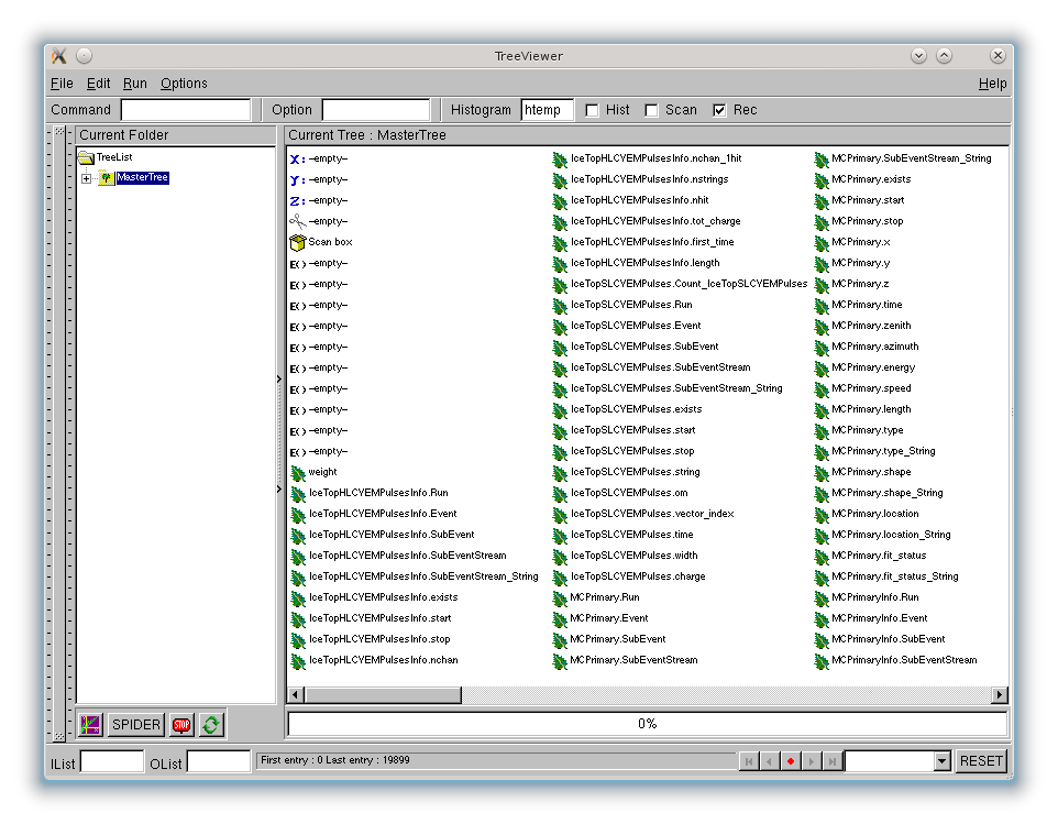
As you can see, all the other trees show up as if they were branches of MasterTree. The quickest way to create a plot is simply double-clicking a branch in this viewer.
Rootwriter TTrees are completely flat. Thus, each branch contains only one leaf. However, branches can be arrays, either of fixed length (e.g. for filter masks: condition_passed and prescale_passed) or variable length (e.g. when booking I3RecoPulseSeriesMaps).
Each tree contains at least six branches:
In order to align the trees every tree contains one line for each event. Therefore it is important to always check the value of the branch called exists.
If the object stored in the tree is an array like structure (like e.g. an I3RecoPulseSeriesMap) the data will be stored in variable-length arrays and an additional branch is added to the tree
In case of fixed-length arrays the length is not stored anywhere in the root file, but it is always the same as defined by the I3Converter.
Note
I3FilterResultMapConverter creates one branch for each filter. Each of these branches is an array of two bools. The first one for the condition_passed flag, the second one for prescale_passed.
In some cases, fixed and variable-length arrays are combined. For instance, when booking ATWD waveforms, a branch of type double[Count_<tree_name>][128] will be created. Each entry will be an array of 128 doubles.
Note
To workaround issues with ROOT’s interpretation of branch types, rootwriter will replace all arrays (not single values) of type char or unsigned char with arrays of int16_t or uint16_t, respectively. Thus, the tree structure might differ from what one would expect from the converter implementation.
Besides opening a TreeViewer you can also use TTree::Print() to get information about the structure of a tree and the stored variable types:
root [3] IceTopHLCVEMPulses->Print();

******************************************************************************
*Tree    :IceTopHLCVEMPulses: IceTopHLCVEMPulses                             *
*Entries :   348915 : Total =       417028258 bytes  File  Size =   89738443 *
*        :          : Tree compression factor =   4.64                       *
******************************************************************************
*Br    0 :Count_IceTopHLCVEMPulses :                                         *
*         | ULong64_t Number of objects in each field                        *
*Entries :   348915 : Total  Size=    2828723 bytes  File Size  =     414516 *
*Baskets :       35 : Basket Size=     386560 bytes  Compression=   6.74     *
*............................................................................*
*Br    1 :Run       : UInt_t run number                                      *
*Entries :   348915 : Total  Size=   18123225 bytes  File Size  =     827981 *
*Baskets :      202 : Basket Size=    2502144 bytes  Compression=  21.85     *
*............................................................................*
*Br    2 :Event     : UInt_t event number                                    *
*Entries :   348915 : Total  Size=   18123641 bytes  File Size  =    2239237 *
*Baskets :      202 : Basket Size=    2502144 bytes  Compression=   8.08     *
*............................................................................*
*Br    3 :SubEvent  : UInt_t sub-event number                                *
*Entries :   348915 : Total  Size=   18124266 bytes  File Size  =     875798 *
*Baskets :      202 : Basket Size=    2502144 bytes  Compression=  20.66     *
*............................................................................*

// etc
Note
MasterTree->Print() will only print the structure of MasterTree, which is probably not what you want. You will have to call Print() on each tree.
The tableio description field is stored in the branch titles. You can retrieve the description of an individual branch as follows:
root [4] IceTopHLCVEMPulses->GetBranch("Event")->GetTitle()
(const char* 0x255e5d8)"event number"
These descriptions are provided by the individual converters and are the same as those stored in the hdf header. Unfortunately, ROOT trees do not have a field where the tableio unit field can be stored.
Of course, the easiest way to create a plot from a tableio root file is using the Draw() method, for instance:
MasterTree->Draw("IceTopHLCVEMPulses.charge");
This will fill all pulses in all events into a histogram.
However, there are more complicated cases, where Draw() and simple cuts are insufficient and you might have to actually loop over the tree by hand.
To do this, assign a variable to the branches you want to inspect and call TTree::GetEntry() inside a loop. For example:
double energy;
MasterTree->SetBranchAddress("MCPrimary.energy", &energy);
for (Long64_t evt = 0; evt < MasterTree->GetEntries(); ++evt) {
    MasterTree->GetEntry(evt);
    // do something with energy
}
For multi-row tables you will need sufficiently large arrays and make use of Count_<tree_name>:
ULong64_t nPulses;
MasterTree->SetBranchAddress("IceTopHLCVEMPulses.Count_IceTopHLCVEMPulses", &nPulses);
double charge[MAX_PULSES];    // set MAX_PULSES to a number large enough for any event you might encounter
MasterTree->SetBranchAddress("IceTopHLCVEMPulses.charge", charge);  // no & before charge!
for (Long64_t evt = 0; evt < MasterTree->GetEntries(); ++evt) {
    MasterTree->GetEntry(evt);
    for (int i = 0; i < nPulses; ++i) {
        // do something with charge[i]
    }
}
Warning
You might be tempted to simplify this task using TTree::MakeClass(). However, this can lead to undesired behaviour for multi-row tables. TTree::MakeClass() will allocate arrays for these tables whose length is inferred from the longest array occurring in the file used when running TTree::MakeClass(). If you then use the resulting code to read other files, longer arrays can lead to crashes through segmentation faults.
When using this approach you need to know the types of branches created by converters. The easiest way to find out (besides checking the code) is TTree::Print() as described above.
PyROOT offers several ways to read data from root trees. In order to work with pyROOT simply import the ROOT module and open a file:
import ROOT

f = ROOT.TFile('output.root')
tree = f.MasterTree
Just like in C++ you can then use TTree.Draw() to create histograms:
tree.Draw("log10(MCPrimary.energy)")
Looping over trees is a little simpler in python. All branches of a tree can be access as attributes of the tree. TTrees are iterable just as branches that contain arrays. PyROOT will automatically make sure that all loops are stopped in time. You do not have to care about the Count_<tree_name> branch.
An example:
for event in f.IceTopHLCVEMPulses:
    for charge in event.charge:
        # do something with charge
Unfortunately, this is relatively slow.
Note
While branches are accessible as attributes of a tree, friend trees are not. Thus code like MasterTree.IceTopHLCVEMPulses.charge will not work.
A faster way to loop over trees is to assign variables to branches just as in C++. In Python this is only possible using array.array or numpy.array because you have to pass a pointer to a fixed-type variable to TTree.SetBranchAddress().
Here is a simple example using numpy.arrays:
import ROOT
import numpy as n

f=ROOT.TFile('output.root')
t=f.MasterTree

energy = n.array([0], dtype=n.double)
t.SetBranchAddress('MCPrimary.energy', energy)

for evt in range(t.GetEntries()):
    t.GetEntry(evt)
    # do something with energy[0], e.g.
    print energy[0]
In the same way you can also read arrays stored in trees. However, you will have to know in advance how many entries you will expect. Let’s add to the example above:
count = n.array([0], dtype=n.uint64)
MAX_PULSES=324       # for IceTop this is enough
charge = n.zeros(MAX_PULSES, dtype=n.double)

t.SetBranchAddress('IceTopHLCVEMPulses.Count_IceTopHLCVEMPulses', count)
t.SetBranchAddress('IceTopHLCVEMPulses.charge', charge)

for evt in range(t.GetEntries()):
    t.GetEntry(evt)
    for q in range(count[0]):
        # do something with charge, e.g.
        print charge[q]
The obvious disadvantage of this way is that you have to write just as much code as in C++.
I3FilterResultMapConverter creates a branch containing an array of two bools for each filter. The first of these two bools stores the condition_passed flag, the second one the prescale_passed flag. So to determine the rate of a filter (e.g. for comparison with monitoring data) you have to look at only one of them, namely the second one, for example:
MasterTree->Draw("FilterMask.IceTopSTA3_11[1]")