IC79 crab flare analysis with IC79 solar WIMP cuts:
short overview:
For section on additionally requested material, click here.The claimed enhanced flux in the Crab Flare may only extend up to a few TeV. Therefore, an analysis that is sensitive to lower ν-energies seems of special interest. The declination of the crab is equivalent to the sweet spot of the solar WIMP analysis, ~23° below the horizon. A solar WIMP analysis targets especially ν's around and below 1 TeV. Cuts for the currently ongoing IC79 solar WIMP analysis were designed and tested for a IC86 sensitivity study for solar WIMPs and are additionally based on knowledge and experience from the IC22 solar WIMP analysis, published in PRL. Consequently, the current IC79 WIMP analysis cuts were applied for the case of the fast-analysis of the crab-flare.
cut levels:
The starting point of this analysis is the online L2 filtered data. No further offline pulse extraction or track fitting was applied. Also for more information on how online L2 data looks like and further data/MC checks and general information on the crab flare and the point-source cut selection, see [ Crab Flare Wiki ]. All files which were used in this analysis can be found under /data/ana/IC79/exp/onlineL2/.
L2b:
A simple "or" cut on the two high-level reconstructions within the onlineL2 processing was applied within a 25 degree zenith band around the crab location. Data/MC agreement for cut level L2b for analysis relevant variables can be found [ L2b ].
L3:
In preparation for the multivariate analysis step in L4 it is important to remove some tails in distributions. Additionally, L3 cuts are chosen to favor track topologies of horizontal tracks within IceCube with a decent quality.
Data/MC agreement for cut level L3 for analysis relevant variables can be found [ L3 ].
TMVA variables; multivariate analysis step:
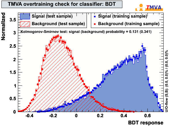
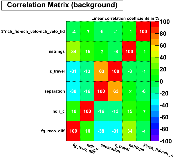
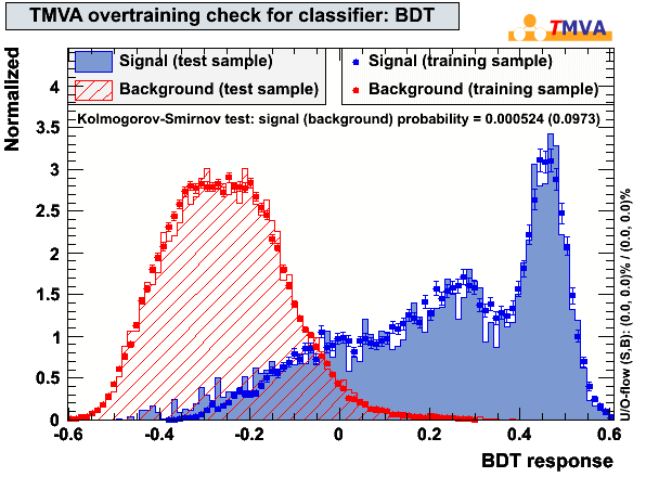
In cut level L4, two BDTs were trained and tested separately. The first BDT has 6 input variables and the second BDT 5. The variables were selected to be uncorrelated in background. The output of BDT1 and BDT2 is multiplied and one single cut is performed in L4 on the output parameter BDT1xBDT2. The input signal to train the BDTs was chosen to be an E-3 muon neutrino spectrum within +- 2.5° within the zenith direction of the crab. The background sample consists of IC79 data. Both training and testing samples consistent of 40000 events and all events are discarded in further analysis step in order to avoid bias.
| BDT input variables | BDT output plot | Overtraining check | Input distributions | Correlation matrix Bg | |
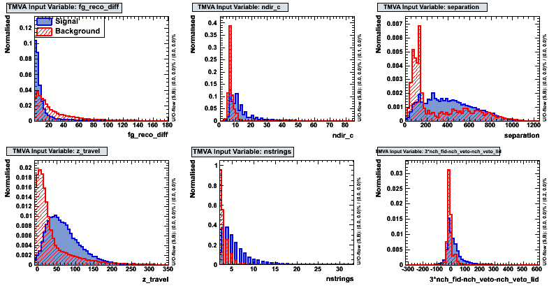
| BDT 1 | firstGuess_MPEFit_reco_difference | 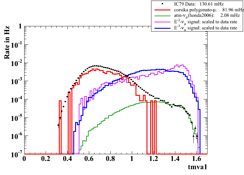 |
 |
 |
 |
| ndir_c | |||||
| separation | |||||
| z_travel | |||||
| nstrings | |||||
| 3*nch_fidutial-nch_veto-nch_veto_lid | |||||
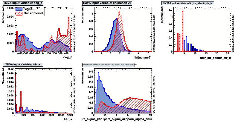
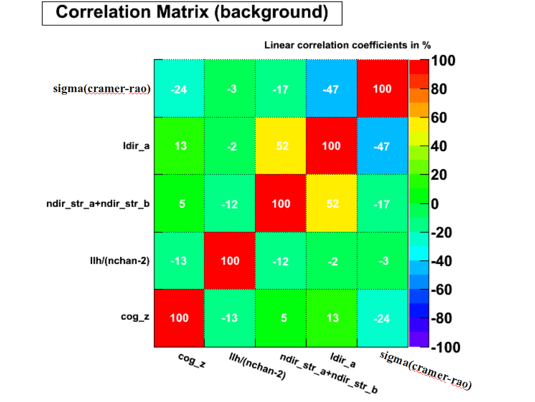
| BDT 2 | σ(cramer_rao) |  |
 |
 |
 |
| cog_z | |||||
| llh/(nchan-2) | |||||
| ndir_str_a+ndir_str_b | |||||
| ldir_a | |||||
L4-final:
The final cut level consists of a simple cut on the (BDT1 x BDT2) variable that was determined by maximizing the expected sensitivity depending on the BDT cut using the point source Llh-code. Additionally, the zenith band around the crab location was reduced to +- 10° to match the final sample of the Madison-point-source cut selection. Data/MC agreement at final cut level L4 for analysis relevant variables can be found [ L4 FINAL ].
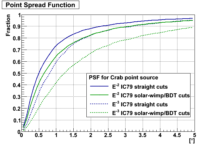
Sensitivities:
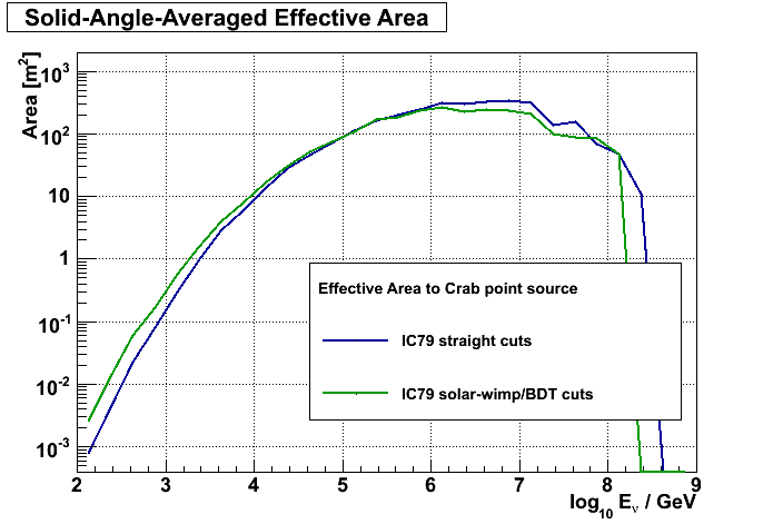
The following 2 plots show the effective area plot as well as the accumulative point spread function for this analysis compared to the point source cut selection.
additionally requested information and answers:
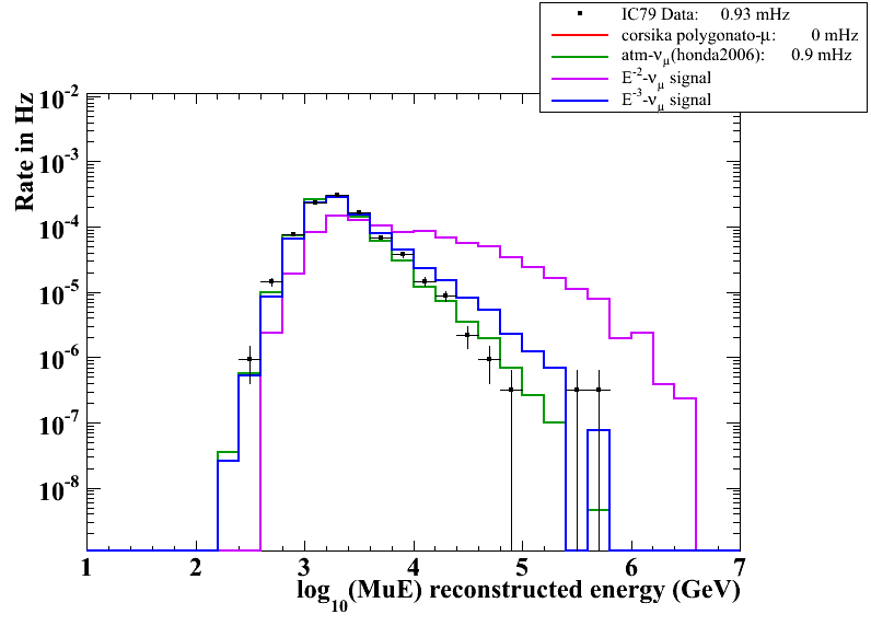
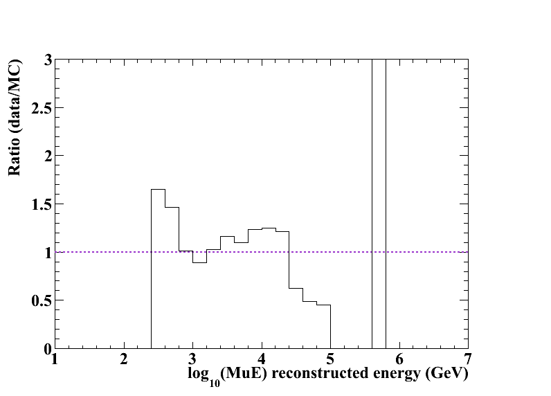
(1) MuEFit Energy distribution at final cut level: (Sirin)
The following to plots show the distributions of the reconstructed energy log10(MuE) at final cut level (left) and the ratio plot for the data/MC comparison (right).
(2) Why 2 BDT's? (Levent)
There is a simple answer that might seem a bit poorly motivated. It works by far the best considering the variables used and available statistics to train and test the BDTs. So, I have 6 and 5 variables in my BDTs, that are all quite powerful in separating Bg from signal. By using all of them in one BDT on gets an 11 dim space, that needs extremely high statistics. Having each BDT with around 5 variables makes them much more stable. This is also not the first time that I used these variables in a multivariate analysis step within an analysis. Most equivalent to this case is a sensitivity study for IC86 solar WIMPs, where I essentially used the same variables.(solar WIMPs)
(3) And how did you select which variable goes into which? (Levent)
Firstly, one selects naturally the strongest(separation power between signal & Bg) variables. Secondly, the BDTs are selected in a way that all variables have not too high correlation for Bg. There is no real value of correlation, where on says you can't get over this or that. As long as the used variable that seems a bit higher correlated, has uncorrelated separation power in some part of the variable space that is well understood by the analyser. But a usual value is around 0.5 or 50% within the correlation matrix. Additionally, these are variables classifying track-reconstruction quality and also exploiting topological features of horizontal tracks within the detector array to separate Muon-Bg from signal (as the crab declination is just below the horizon).
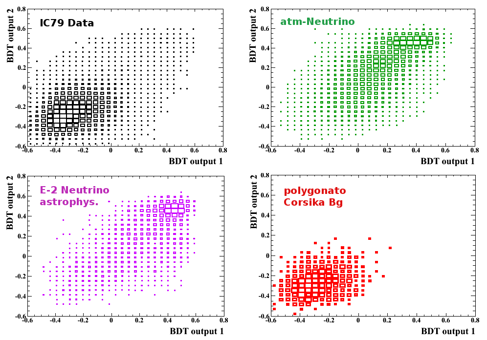
(4) Have you tried combining all variables into one BDT, and how much worse was it? (Levent)
Yes, I tried this. First I used all 11 and then of course re-optimised this particular BDT and ended up with 9 variables I think. I don't have quantitative numbers to directly compare any-more, but they were roughly 30-40% worse. To be a bit more precise, I needed to cut much harder in order to be able to achieve a similar atm.nu purity in the remaining data. Please also see the following plot, showing the BDT-output values in a 2-dimensional scatter plot. There you can see how the events are distributed in the 2D output space. This might also illustrate some of the other answers a bit better.
(5) BDT optimisation: Did you play with the BDT parameters, nTree, nCuts, pruning yes/no? (Levent)
Yes I did. nTrees is quite optimal with the default value of 400. I optimised a lot during the WIMP sensitivity study with these values. The pruning turned out to be of extreme importance in this case in improving the performance of the BDTs. As this analysis uses real data as Bg (that of course contains atm-nu as a signal like component) a better performance was achieved in setting the pruning value a bit higher than I used to do when I was training with Corsika as Bg.
(6) Variable selection: Have you tried classifying the variables used according to their cut strength? Train the BDT's with one variable omitted to see how much you loose in cut strength or signal efficiency? E.g., in your first BDT, ztravel and seperation show the highest correlation, did you try removing one of the variables? Same goes for the second BDT with ldir_a and ndir_str_a + ndir_str_b: (Levent)
Your question describes pretty well the process of optimising a BDT. I knew from previous studies of course which variables are powerful and which have less strength, but adding removing and evaluating for each different scenario the BDT output is the only reliable method to optimise the BDT. As you may know, the BDT itself categorises before and after training variables according to their cut strength. But this is a bit misleading and should not be used as the only method to determine whether a variable is stronger or weaker than others. As an example: If a variable is changing rapidly within short range, the BDT will take it more often to split the tree within this section, as it changes very quickly. The cut-strength given by the BDT is a measure on how often the variable is used to make a cut. Hence, such a variable is used very often due to the spectral feature, but not because it is powerful. About the specific variables you mention in your question. Yes, I removed them and added them one by one, and the obtained selection was found to be the best.
(7) final cut level: Can you shows a plot of the MRF or MDP as a function of the cut strength? (Levent)
Sorry, I can't. The cut was chosen in a simple way using the point-source-LLH method of calculating sensitivities and discovery potentials (together with Chad F.). We increased in small steps the final cut from a very loose starting value, and evaluated the discovery potential with the LLH method. The cut were we found the corresponding minimal Flux with the LLH was used to set the final L4 cut. I did not save the fluxes with increasing L4-cut-value, so I cannot provide a plot in the moment.
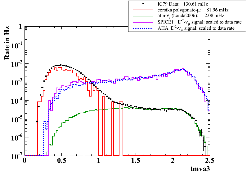
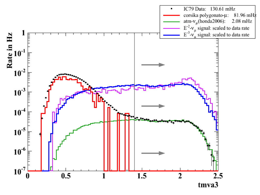
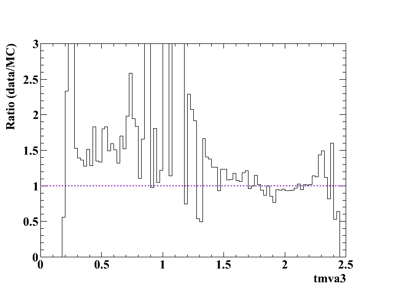
(8) For plot http://icecube.wisc.edu/~mda65/crab/plots/tmva3_L3_tmva_fixed.png, I would like to see the ratio between data and (crs+atm nu): (Levent)
Please see requested plot below next to the plot mentioned in your question.
(9) Systematic study with signal simulation using AHA-icemodel: (Kurt)
The nugen simulation (with AHA-icemodel) is processed through the analysis chain and an example plot, showing the last cut on the combined BDT output, can be found below. The processed files are also given to Mike & Juanan for actual sensitivity calculations and potential effective area plots. (Further information on this on the wiki or soon below). Both signal simulations seem to be consistent with each other in the L4 selected parameter region.