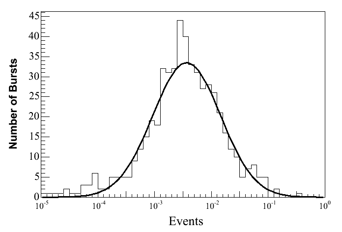

Distribution of expected events from
actual BATSE bursts
Cut Selection Based on Model
Discovery Potential
Since
the sensitivity of this analysis to conventional GRBs will be above
that of previous AMANDA analyses, it was decided to optimize for
discovery (although it turns out that the sensitivity we obtain at cuts
based on discovery is not much different than what one obtains from the
MRF). In precise terms, optimizing for discovery in this case
means
finding the cuts such that we have a 90% of getting a signal with at
least 5 sigma significance at the lowest possible flux. Model
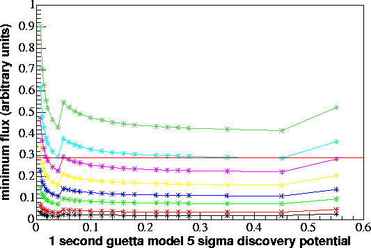
Discovery Potential plots for both searches are shown below, with event
distributions modeled by the afforementioned "Guetta"
distribution.
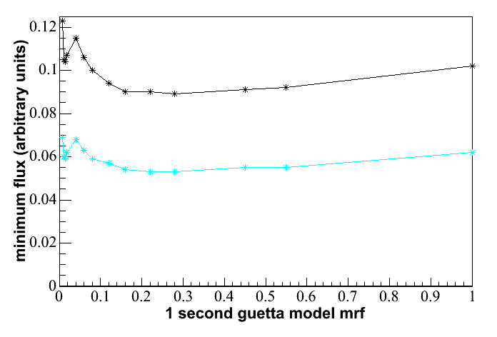
The x-axis shows SVM cost factor (equivalent to tightness of cuts at
the final level) with tighter cuts on the left of the plot and looser
cuts on the right. The y-axis shows the minimum flux (in average
events per burst) one needs to have a certain percent chance to see a
signal with at least 5 sigma significance. For example, the light
blue
line shows the minimum signal flux one would need at each cost factor
to have a 90% chance of seeing a 5 sigma signal. While the 90%
line
was the one selected to base cuts on, one obtains very similar results
foor anything above 25%. The cuts selected based on these two
plots
are cost factor .08 (80.9% signal retention) for the 100 second search
and .45 (96% signal retention) for the 1 second search, although these
are very close to the minima at smaller cost factors, which would
require fewer events for a 5 sigma detection, but also cut away a
larger percentage of the signal. (The horizontal red line is
drawn on the 1 second plot to demonstrate that .45 really gives the
minimum, albeit by a small margin.)
f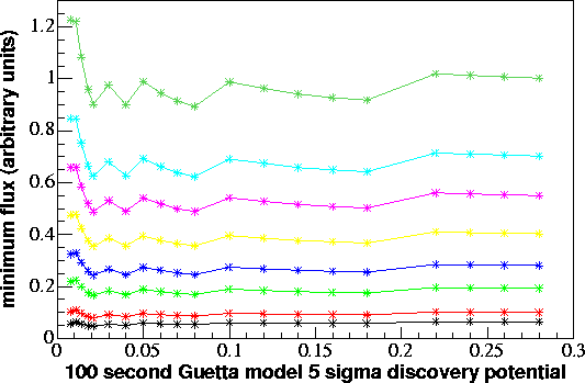
Statistical
power: dark green - 99%, light blue - 90%, violet - 75%, yellow
- 50%, blue - 25%, light green - 10%, red - 1%, black - 0.1%
Model
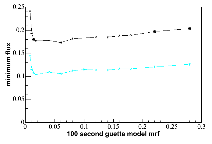
Rejection Potentail plots obtained
using the "Guetta" distribution are shown below. Again, cost
factor
(equivalent to tightness of cuts) is shown on the x-axis. The mrf
at
the cut levels selected by the Model Discovery Potential method are
only 7.7% above the minimum in the case of the 100 second search and
3.2% above the minimum in the case of the 1 second search, so in this
case there turns out not to be much difference between optimizing for
limit setting and optimizing for discovery.
Comparison
With Other Ways of Distributing Events Among Bursts
| 100 second search minimum |
% diff between minimum and
selected cut |
1 second search minimum |
% diff between minimum and
selected cut |
|
| Guetta Distribution |
||||
| 3 sigma |
0.08 |
0% |
0.55 |
1.1% |
| 4 sigma |
0.04 |
2.7% |
0.16 |
28.6% |
| 5 sigma |
0.08 |
0% |
0.45 |
0% |
| MRF |
0.018 |
7.7% |
0.28 |
3.8% |
| Single Burst |
||||
| 3 sigma |
0.08 |
0% |
0.55 |
0.7% |
| 4 sigma |
0.08, 0.18 |
0% |
0.16 |
11.4% |
| 5 sigma |
0.18 |
1.3% |
0.45 |
0% |
| MRF |
0.08 |
0% |
0.35 |
1.9% |
| Flat Distribution |
||||
| 3 sigma |
0.014 |
29.5% |
0.04 |
40.7% |
| 4 sigma |
0.018 |
23.1% |
0.014 |
54.3% |
| 5 sigma |
0.021 |
16.2% |
0.04 |
12.9% |
| MRF |
0.014 |
30.0% |
0.014 |
20.1% |