Simulating the atmospheric neutrino flux with CORSIKA

Up to now IceCube has simulated atmsopheric neutrinos by generating a power-law flux and weighting it to a parameterization of the atmospheric neutrino flux. As long as one only selects up-going neutrinos this procedure is as correct as the underlying parameterization, but it is seriously flawed when used to analyze data samples that contain down-going neutrinos. Since atmospheric neutrinos are produced in air showers, at least some of the muons produced in the same air shower will survive to the depth of the detector, making the neutrino event indistinguishable from a muon bundle event and unlikely to survive an event selection that rejects incoming, down-going muons.

This suppression of the “bare” atmospheric neutrino flux is difficult to parameterize, as it depends on the details of the correlations between the neutrino spectrum and the accompanying muon energy spectrum, multiplicity distribution, and radial distribution, as well as the way these interact with a specific event selection. Possibly the best way around this difficulty is to simulate the atmospheric neutrino flux directly, muons and all.

Three major modifications are required to make this practical: biasing CORSIKA to produce a sufficient number of high-energy neutrinos, keeping track of the parent meson of each neutrino, and extending NeutrinoGenerator to pick a neutrino out of the bundle and force it to interact.

The necessary modifications to CORSIKA are in a local git repository, which you can check out via

git clone /net/user/jvansanten/projects/2013/corsika-74000 .

The front-end to NeutrinoGenerator is in the NeutrinoSmasher project.

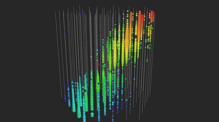
A 2 PeV atmospheric \(\nu_{\mu}\) interacting inside the detector. As a minor detail, it’s buried in the middle of a 4 PeV muon bundle.

Step 1: High-energy neutrinos from CORSIKA

Above \(\sim 1\) TeV, the atmospheric neutrino flux is an image of the input cosmic ray flux \(N_0(E)\) with contributions from the decays of each type of meson produced in the initial interactions of cosmic rays with a nucleus in the atmosphere:

(1)\[\frac{dN_{\nu}}{dE_{\nu}} \propto N_0(E_{\nu}) \sum_{i=\pi, K, \ldots} \frac{A_i}{1+ B_i \frac{E_{\nu}}{E_{crit}}}\]

The \(A_i\) parameterize the meson yield from interactions between cosmic rays and nuclei in the atmosphere, while the \(B_i\) deal with the competition between energy loss and decay. The \(E_{crit}\) are the critical energies for each meson, above which interaction dominates decay. This makes conventional atmospheric neutrinos quite rare above a few tens of TeV. Since CORSIKA samples the final states of hadronic interactions and the decays of mesons at natural frequency, this makes it necessary to simulate a full year of livetime in order to get a handful of atmospheric neutrinos. One way around this limitation is to over-sample the kinds of rare processes that lead to high-energy conventional neutrinos.

The largest suppression in the conventional flux comes from the lifetime of pions and kaons. At 10 TeV, the mean decay length of a charged pion (kaon) is 560 (75) km, making them much more likely to interact and lose energy than to decay and produce neutrinos. In order to produce more high-energy neutrinos in CORSIKA simulation, I artifically reduce the decay depth of the highest-energy meson produced in the first interaction, and compensate for the resulting bias with an appropriate weight.

In CORSIKA, the competition between interaction and decay is modeled by drawing one sample each from the exponential distributions of decay and interaction lengths, and picking the smaller one. The mean decay length is:

\[\lambda \equiv \beta \gamma c \tau\]

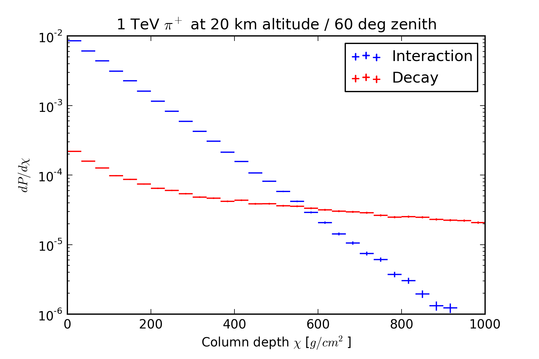
In CORSIKA this is converted to a column depth based on the trajectory through the atmosphere, and then compared to a sample from the exponential distribution of interaction lengths (also as a column depth, with mean \(\Lambda\) that depends on the meson-air cross-section). The conversion between the two units depends on the density profile of the atmosphere, and therefore on the zenith angle of the parent shower and the altitude at which the meson is produced. The figure below shows the distribution of interaction depths for 1 TeV pions produced at 20 km altitude at a zenith angle of 60 degrees, as well as the distribution of decay lengths converted to column depths. The resulting distribution of decay column depths is notably not a simple exponential.

In a curved atmosphere there is no closed-form expression for \(\chi(l)\), but it is at least monotonic, so the quantiles of the distribution of \(\chi\) can be obtained from the quantiles of \(l\) if \(\chi(l)\) can be evaulated numerically. The first quantity of interest is the median decay depth. In order to bias the simulation towards decays, I first calculate a lifetime adjustment \(b\) that makes the median decay depth equal to the median interaction depth:

\[\chi (\frac{\lambda}{b} \ln2 ) = \Lambda \ln2\]

numerically by repeated applications of CORSIKA’s existing column-depth accumulation routine NRANGC. If \(b \leq 1\) the particle is likely to decay without any intervention, and no biasing or weighting is performed for that event.

Given the lifetime adjustment factor, I draw a sample from the exponential distribution of decay lengths for a new lifetime \(\tau/b\), convert it to a column depth, and compare to a sample from the exponential distribution of interaction depths. As in the normal sampling mode, the meson decays if \(\chi_{\rm dec} < \chi_{\rm int}\), and interacts otherwise. However, since I no longer sample decay lengths at natural frequency, I must apply a weight to account for the bias. The probability of decay is

\[\begin{split}P({\rm decay}|\lambda, \Lambda ) = P( \chi(l_{\rm dec}) < \chi_{\rm int} )\end{split}\]

In the case where the particle decays, the appropriate weight is:

\[\begin{split}w_{\rm dec} \equiv \frac{P( \chi(l_{\rm dec}) < \chi_{\rm int} )}{P( \chi(l_{\rm dec}/b) < \chi_{\rm int} )}\end{split}\]

which accounts for the fact that a rare process has been oversampled. If on the other hand it manages to interact, the appropriate weight is:

\[\begin{split}w_{\rm int} \equiv \frac{1-P( \chi(l_{\rm dec}) < \chi_{\rm int} )}{1-P( \chi(l_{\rm dec}/b) < \chi_{\rm int} )}\end{split}\]

which accounts for the fact that a common process has been undersampled. Because of the aforementioned lack of a closed form for \(\chi(l)\) these probabilities have to evaluated by Monte Carlo by repeatedly sampling from the distributions of decay and interaction depths. Since CORSIKA already knows about per-particle weights in its thinning mode, the decay weight is recorded in the WEIGHT field of the meson particle record, and is automatically propagated to its daughters and written to the output file. Since the siblings of the weighted meson are not affected by the biasing scheme, they receive a weight of 1.

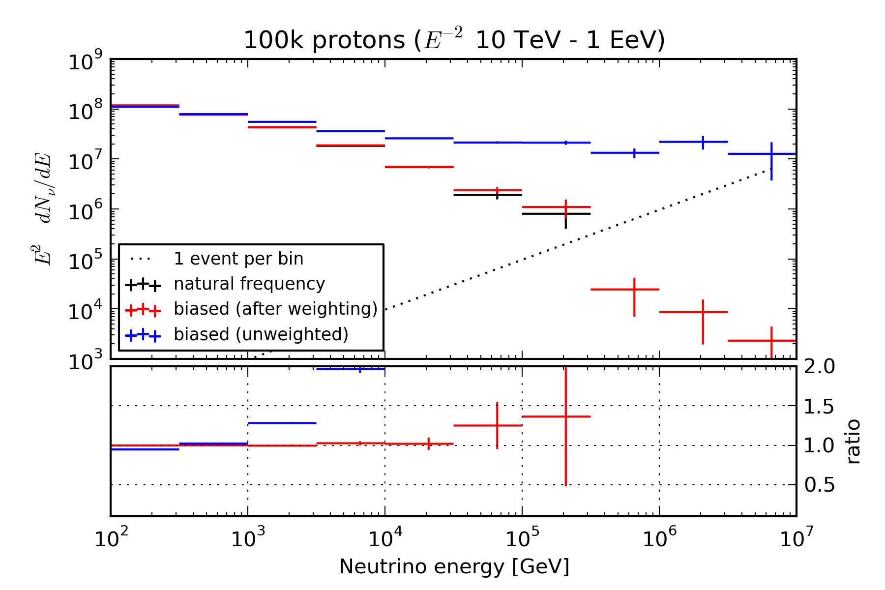
This biasing/weighting scheme produces many more high-energy neutrinos than sampling at natural frequency. In the following example below, 100k proton primaries were simulated on an \(E^{-2}\) spectrum from 10 TeV to 1 EeV, using SIBYLL as a hadronic model. The black histogram in the upper panel shows the energies of neutrinos as produced by CORSIKA v740000; statistics run out at 100 TeV. The blue histogram shows the raw distribution of maximum energies when the simulation is run using the scheme described here; the statistics extend 10x higher in energy and sample event rates that are 1000 times smaller with the same number of simulated events. The red histogram shows the same distribution with weights applied; it matches the un-biased distribution where it has sufficient statistics, and continues the same trend afterward.

Another way of looking at this is use \(E^2 dN/dE\) instead of raw event counts so that the spectrum of injected primaries appears flat. Since this muddles the natural statistical meaning of “1 event,” a dotted line has been added to guide the eye. As can be seen here, the effect of the biasing scheme is to remove the energy dependence of the competition between interaction and decay, making the un-weighted neutrino spectrum an image of the input nucleon spectrum.

Step 2: Tagging parent mesons

The largest uncertainties in the neutrino flux (and associated muons) come from the assumed primary spectrum/composition and the model of high-energy hadronic interactions, in particular the spectrum and production rates of secondary mesons. The latter is most true of the component arising from the decays of charmed mesons, as the forward production rate of charmed mesons cannot be calculated with QCD and is mostly unconstrained by accelerator measurements. Within a given hadronic model, these uncertainties can be approximately taken into account by re-weighting the neutrino and muon fluxes according to the properties of the parent mesons. To do this, however, one needs to be able to determine the energy and type of the parent mesons.

Mainline CORSIKA already implements part of this feature in the EHISTORY option, where the parent and grand-parent of each muon that reaches the observation level are written to the output file if the MUADDI keyword is supplied in the steering file. The local fork linked about extends this with another keyword, NUADDI, which causes the same information to be written for neutrinos.

Step 3: Selecting a neutrino to interact

In its usual mode of operation, NeutrinoGenerator both generates neutrinos and simulates their interactions. This proceeds in the following steps:

1. Generate a neutrino (or anti-neutrino, with 50% probability) of a given flavor, with an energy drawn from a power law spectrum, a direction picked isotropically from the sky, and a position such that it starts at the surface of the Earth, and passes through a circle of fixed radius around the origin of the IceCube coordinate system.
2. Propagate it through the rock and ice to a point near the detector, allowing it to be absorbed in the Earth along the way.
3. Pick an interaction type with probability proportional to the cross-section for that process.
4. Pick an interaction length uniformly on a line segment that passes through the simulation volume, place the daughter particles of the interaction there.
5. Calculate a weight that accounts for both (a) the probability that the neutrino would have interacted after the chosen length at natural frequency and (b) the generated fluence of neutrinos of the chosen energy.

To re-use the bits of NeutrinoGenerator that implement neutrino cross-sections, we need to pry this sequence apart. Given a bundle of muons and neutrinos from CORSIKA, we only need to pick a neutrino and then force an interaction.

Select a neutrino

Just like muons, high-energy atmospheric neutrinos typically come in bundles. However, it is extremely unlikely that they will all interact, so we have to pick a single one to force to interact and calculate a weight that compenstates for the selection bias. The simplest possible approach is to take each neutrino in turn, in which case the weight for each event is 1. If, on the other hand, we want to use each event only once, we could pick one at random (with probability \(p_{nat} \equiv \frac{1}{N}\)) and assign it a weight of \(N\), which accounts for the fact that it is representative of the population it was drawn from. However, we will usually be interested in the highest-energy neutrino in the bundle, and so will bias the selection by energy raised to some power. If instead we pick a neutrino with probabilility

\[p_{sel,i} \equiv \frac{E^{\gamma}_i}{\sum_i E^{\gamma}_i}\]

then the selection weight for the event is

\[w_{sel} \equiv N \frac{p_{nat}}{p_{sel,i}} = \frac{1}{p_{sel,i}}\]

This has the desired behavior: if a given neutrino has a very high selection probability then the selection weight is nearly 1 (since the neutrino is representative only of itself, not the population it was drawn from), but if the selection probability is small then it will be weighted up.

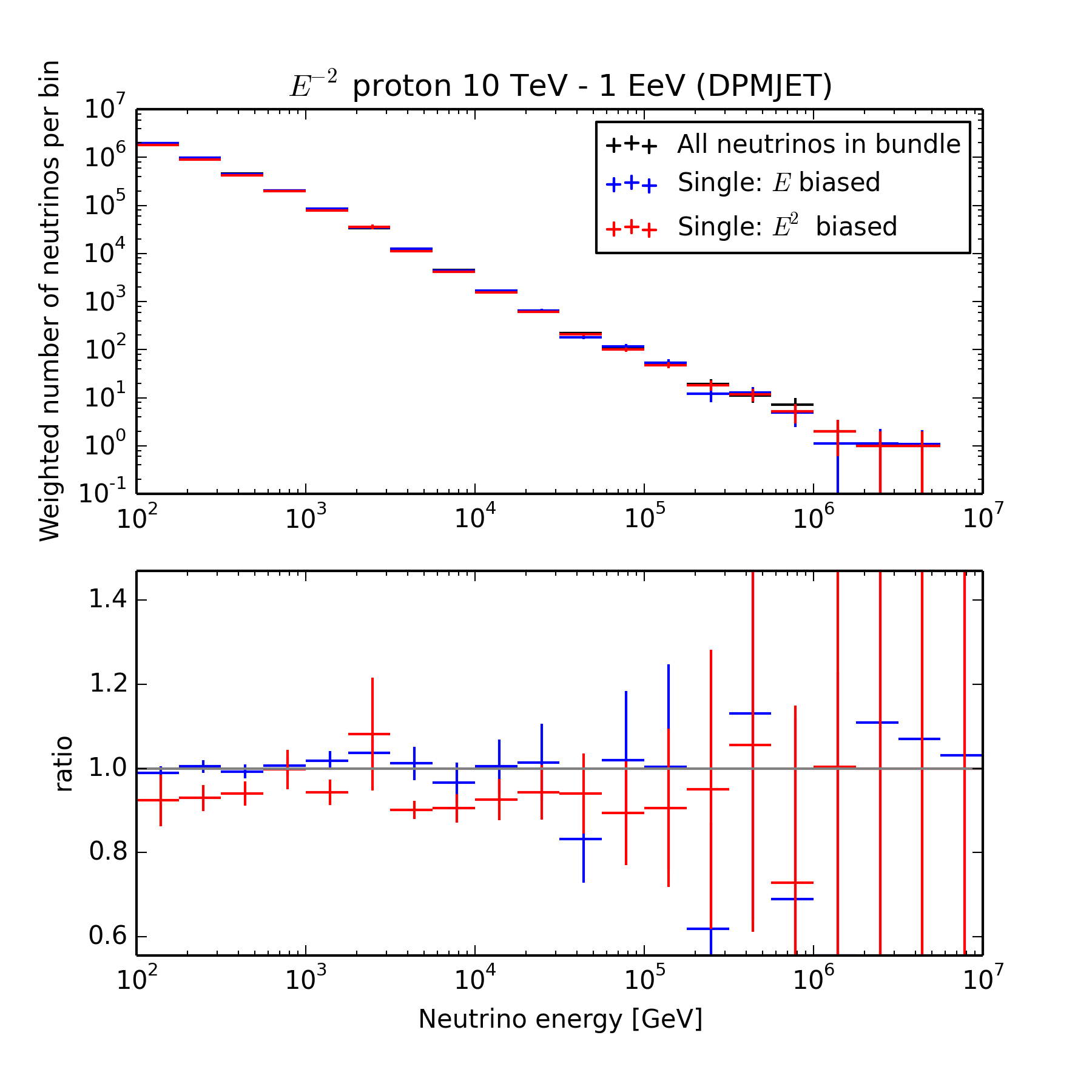
This scheme is implemented in the SourceSelector module, which selects a neutrino, records the selection weight, and removes non-selected neutrinos from the MCTree. The figure below shows the inclusive spectrum of neutrino energies obtained in three modes:

1. Over-sampling: each neutrino in the bundle is selected in turn
2. Biased: exactly one neutrino is selected, with a probability proportional to the fraction of the total neutrino energy it carries
3. Biased: same as (2), but biased by \(E^2\) rather than \(E\)

The \(E\)-biased selection reproduces the over-sampled distribution well, albeit with higher variance since it has 5 times fewer entries. The \(E^2\) bias is too strong, as it causes lower-energy neutrinos to almost never be selected, and results in underestimation of the rate below 100 TeV.

Force an interaction

In its usual mode of operation, NeutrinoGenerator uses an axial cylinder of 1200 m radius as a target surface. While this makes the geometry and weighting calculation simple when starting directions are chosen uniformly in solid angle, it is not a particularly efficient way to select neutrino trajectories that pass through the detector. This is especially true when using CORSIKA to generate neutrinos, since CORSIKA is capable of drawing the zenith angles of primaries in proportion to the projected area of an upright cylinder, and I3CORSIKAReader places showers so that the axis passes through a point in an upright cylinder centered on the detector. Since we’re only interested in things that pass through that same target cylinder, we can choose an interaction position inside the cylinder. The usual volume extension to account for muon range can be implemented by moving the first possible interaction point from the cylinder surface backwards along the neutrino direction. This takes care of steps 2 through 5a.

In order to avoid re-writing all of the I3MCTree manipulation routines, the interaction-forcing is implemented as an I3PropagatorService called NeutrinoProagator.