Overview
1st data cleaning is designed to ‘remove’ 1) unphysical waveform/event caused by DAQ error, and 2) the cuts that reducing livetime
Time period that contaminated by weather balloon also removed from live time by cross-checking with balloon’s GPS log (CW GPS cut)
Most of the cuts are designed to remove the event by only checking DAQ reading
IRS block index, SensorHk reading, Event rate
All the cuts are independant.
This cut was applied to blinded (100%) data to produce accurate pedestal
1st data cleaning is done by below command:
source ../setup.sh
python3 script_executor.py -k sub_info -s <station ID> -r <run number> -b 1          # collect sencondary information
python3 script_executor.py -k qual_cut_1st -s <station ID> -r <run number> -b 1 -q 1 # performs 1st data cleaning
It will use pre_qual_cut_loader and ped_qual_cut_loader class
DAQ index cut
This cut is done by get_daq_structure_errors function
It is designed to remove unphysical event by checking secondary information (DAQ index)
Corrupted IRS block / DDA board / channel masking index and unexpected WF length has strong correlation with unphysical WF shape
Number of bad events identified by DAQ index cut is negligible in live time (rare event)
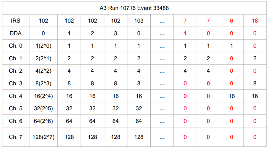
Fig. 14 secondary index of DAQ error event
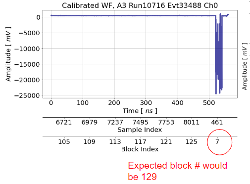
Fig. 15 DAQ error wf with block and sample index
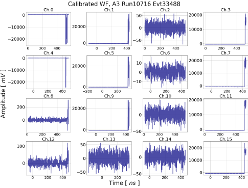
Fig. 16 DAQ error 16 wfs with block and sample index
DAQ index cut will test each event’s DAQ reading by below categories
number of IRS blocks are always 4 multiples
IRS number is always the same for all DDAs
DDA index is always like 0,1,2,3,0,1~
Channel masking is always ‘1’ for all 8 binary digits
There is a block gap or not
WF length is always same or greater than run configuration. example) soft:8, RF/Cal:28, (depending on DAQ configuration)
Cut 5 & 6 are imported from previous A2/3 diffuse analysis
First minute cut
Related doc. DB2554
This cut is done by get_first_minute_events function
The events at every beginning of the run have unphysical WF shape, such as Spikey WF, large offset with a pedestal
Cause is unknown. It might be due to digitizer reset issue
This cut will exclude first 1 minute of every runs
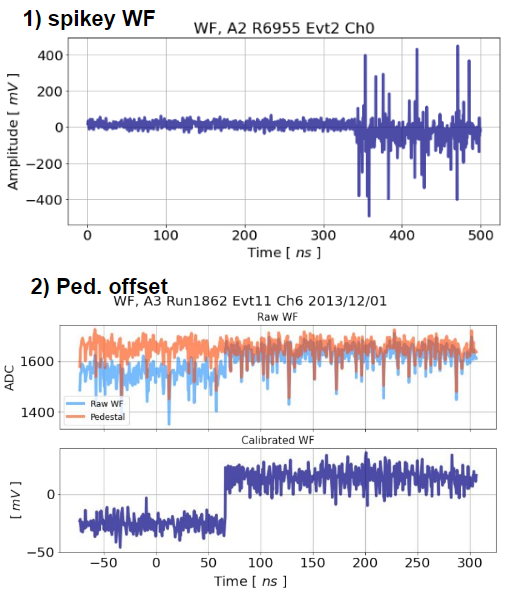
Fig. 17 bad wf in first minute
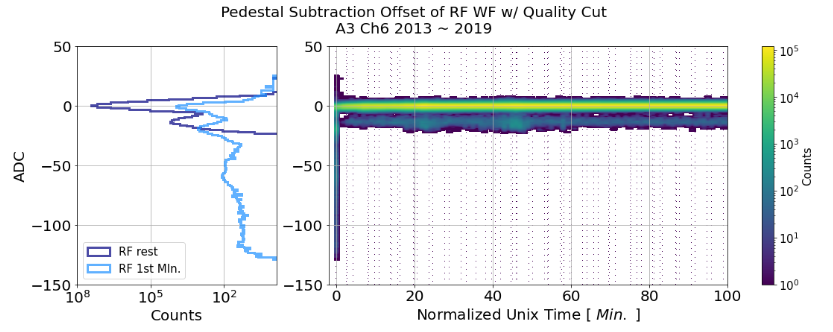
Fig. 18 distribution of first minute wfs in median
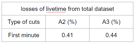
Fig. 19 livetime losses of first minute cut
DDA voltage cut
Related doc. DB2530
This cut is done by get_bias_voltage_events and get_bad_evt_rate_events function
Unstable bias voltage feeds on the DDA boards cause unphysical WF.
Shift of Noise level, 0 ADC event, time drift, and 0 Calpulser rate
If DDA voltage readings (in sensorHk) were out of 3 ~ 3.5 or Calpulser rate was lower than 0.85 Hz, events are removed
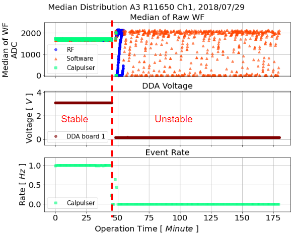
Fig. 20 data status with sensoeHk data
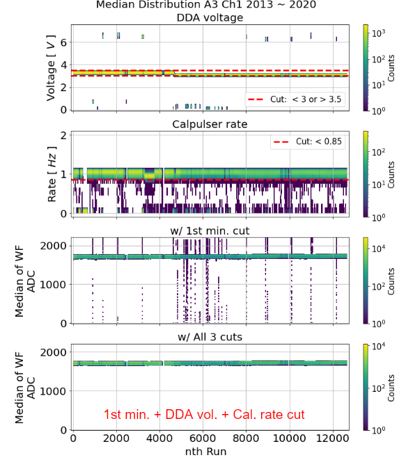
Fig. 21 result of the cut
High software rate cut
Related doc. DB2554
This cut is done by get_bad_evt_rate_events function with use_sec = True option
High Software rate are presented mostly beginning of the run
Assuming DAQ / internal clock are not performing well
If there is more than 2 software event per unix time, all the events in that unix time are removed
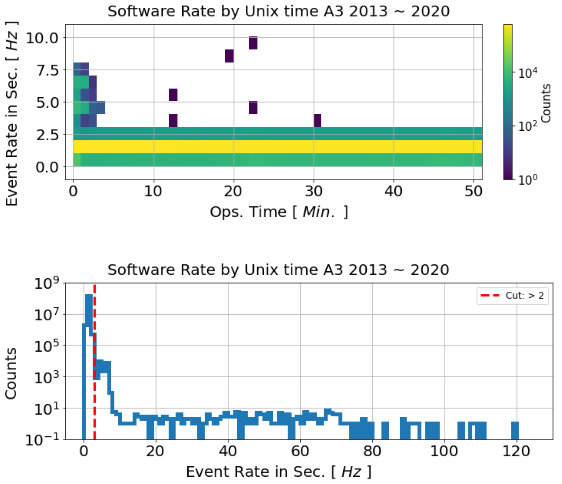
Fig. 22 distribution of software rate. top: based on operation time, bottom: baseed on rate
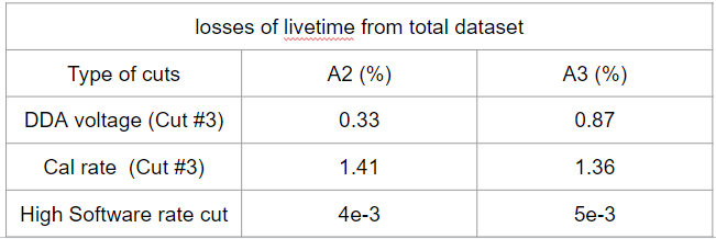
Fig. 23 livetime losses of DDA voltage and high software cut
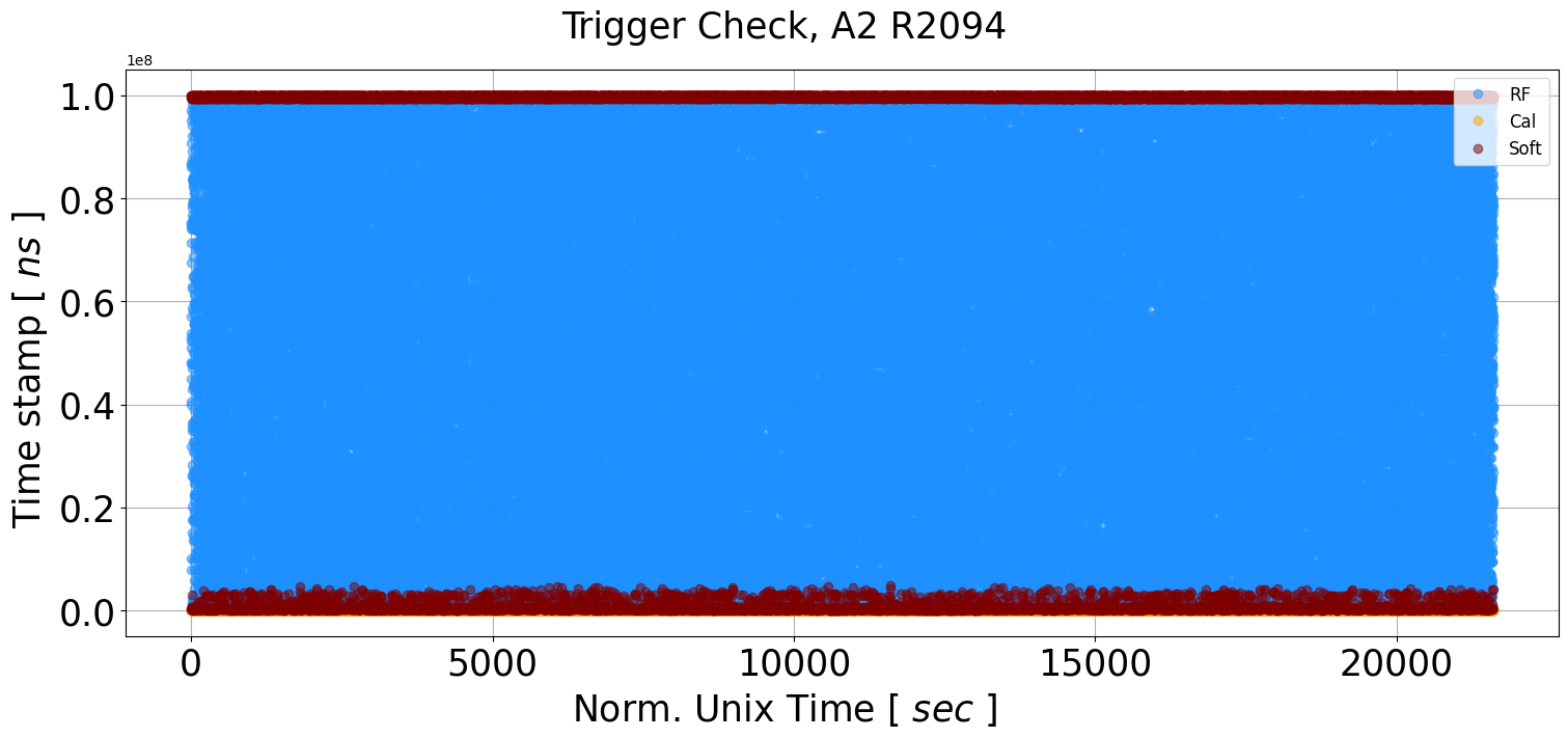
Fig. 24 example run when software rate is 2
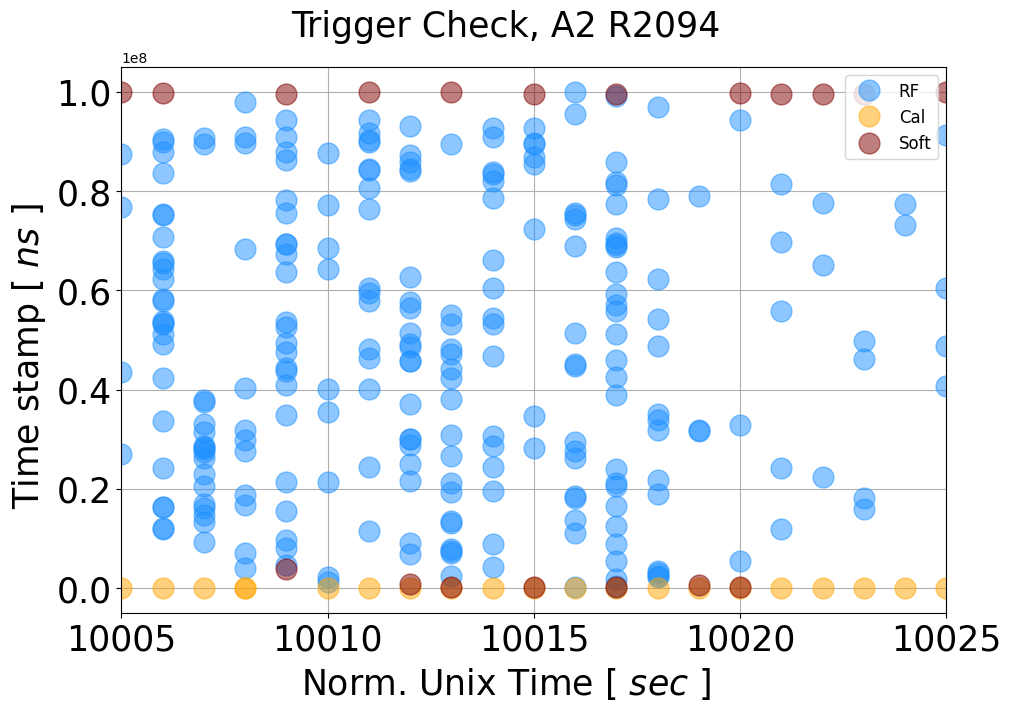
Fig. 25 example run when software rate is 2. Maroon circle indicates software triggered event.
Short run cut
Related doc. DB2560
This cut is done by get_short_run_events function
Decided to remove the run if Ops. time is shorter than 30 min. or number of RF/Soft events are smaller than 10000
Focus the analysis to the run that has normalish Ops. time
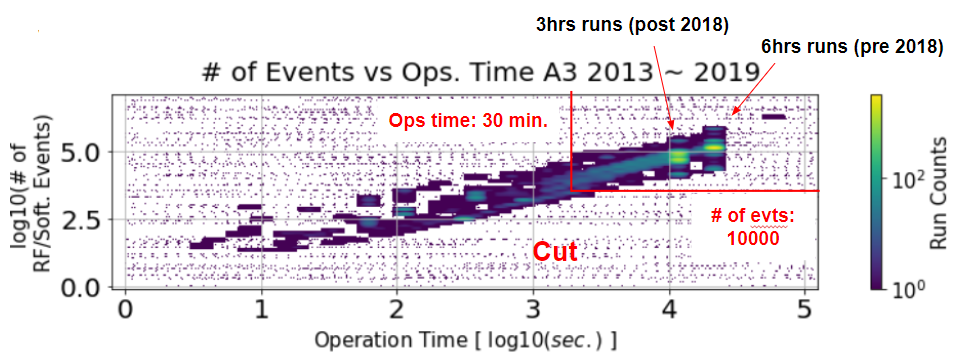
Fig. 26 distribution of runs based on operation time and number triggered events
Known bad runs / unix time cut
This cut is done by get_known_bad_unix_time_events and get_known_bad_run_events function
Most of known bad runs / unix times are corresponding to calibration run or surface activity during the pole season
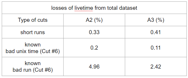
Fig. 27 livetime losses of short run, known bad run and bad unix time
CW GPS cut
Related doc. DB2664
This cut is done by get_cw_log_events function
The event that has weather balloon signature is removed by MET’s balloon flight log
If distance between station and balloon is smaller than ~17 km, events in that period are removed
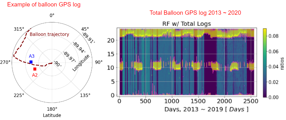
Fig. 28 example GPS path and overlap with Sinesubtract data
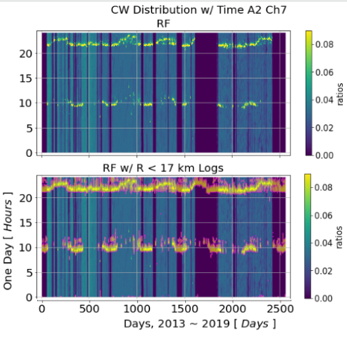
Fig. 29 total comaprison 2013 to 2020
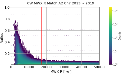
Fig. 30 Sinesubtract data vs distance between station and balloon
Pedestal cut
Related doc. DB2560
This cut is done by run_ped_qual_cut function
If the run has a short operation time or small number of triggered events, It has not good enough events to create a pedestal for all buffer regions
After all the cuts, If usage of any IRS block was below 20 (current Config. file limit for pedestal production), run will be removed
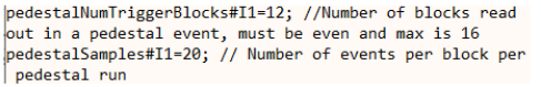
Fig. 31 pedestal configuration in the log file
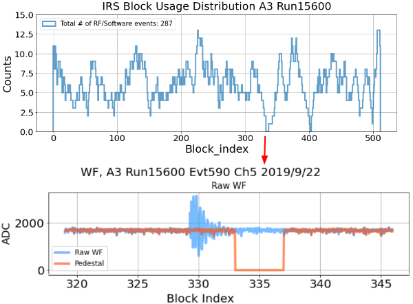
Fig. 32 example of bad pedestal file
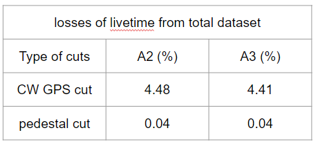
Fig. 33 livetime losses of CW GPS cut and pedestal cut
Livetime
Total livetime after 8 cuts (Good livetime)
A2: 5.45 -> 4.85 years (88.95 %)
A3: 5.27 -> 4.79 years (90.91 %)
~5% from CW GPS, ~4% from known bad runs, and ~1% from the DAQ error.
Simulation results are weighted based on ‘Good’ live time
This plot is done by dat_summary_live.py, dat_summary_live_sum.py and Check_Sim_v34.0.5_live_time_plot script
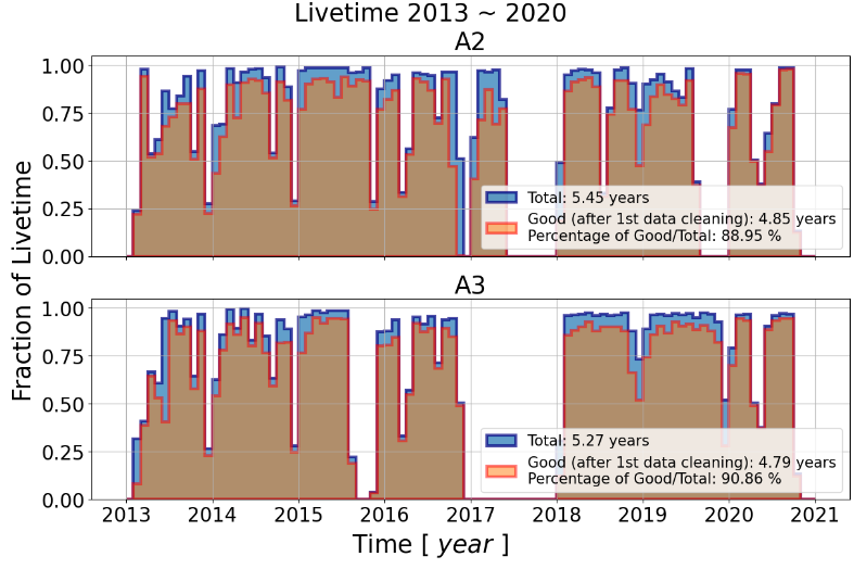
Fig. 34 live time after 8 cuts
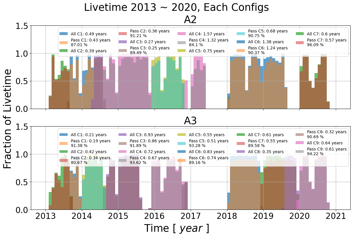
Fig. 35 live time after 8 cuts per configuration
Pedestal production
Pedestal production is done by repeder
Default pedestal measured from DAQ has a offset and causes miscalibration
new method is extracting pedestal from ADC itself
Aligning raw data (ADC) with their analog buffer index and calculates median value of each analog buffer cell
pedestal production is done by below command:
source ../setup.sh
python3 script_executor.py -k ped -s <station ID> -r <run number> -b 1               # produces pedestal
It will launch repeder in AraRoot
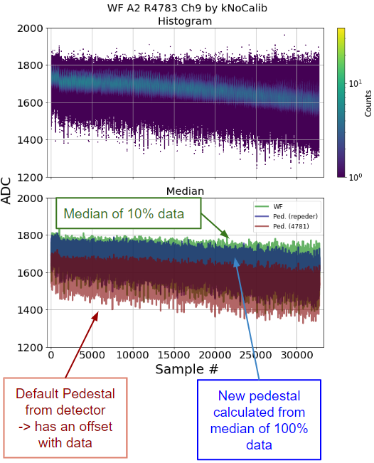
Fig. 36 comparison between default and repeder
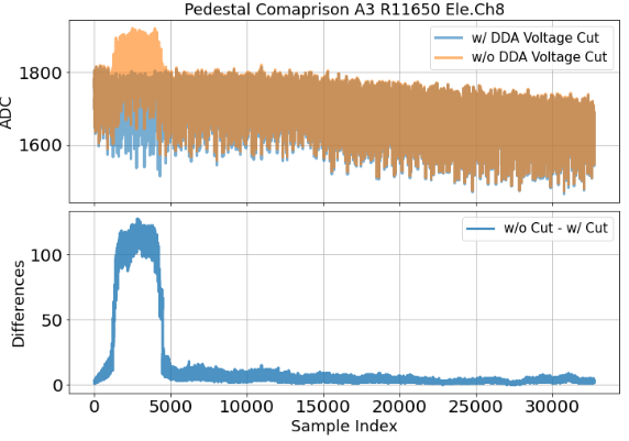
Fig. 37 In this run, unphysical WFs are clustered in the X: 0 ~ 5000, Y: 2000 regions more than normal WFs. So, the median calculation in repeder chosen unphysical WF cluster as an expected baseline of run
L1 cut (potential cut)
This cut is living in the package. But I decided to exclude from 1st data cleaning
It is designed to remove the period that trigger is stablizing to servo goal value
Reason I decied to excluded it are 1) The event that removed by this cut is not that much different with thermal noise event and 2) It is taking out 15 % of live time
But we must explore this period further in the future
This is done by get_bad_l1_rate_events function
Low RF rate cut
Every beginning of the run, low RF rates are observed while threshold is stabilizing itself
Decided to removed all events when RF event rates are low
But this can be re-defined by threshold value (the hardware value), not by empirical cut !!
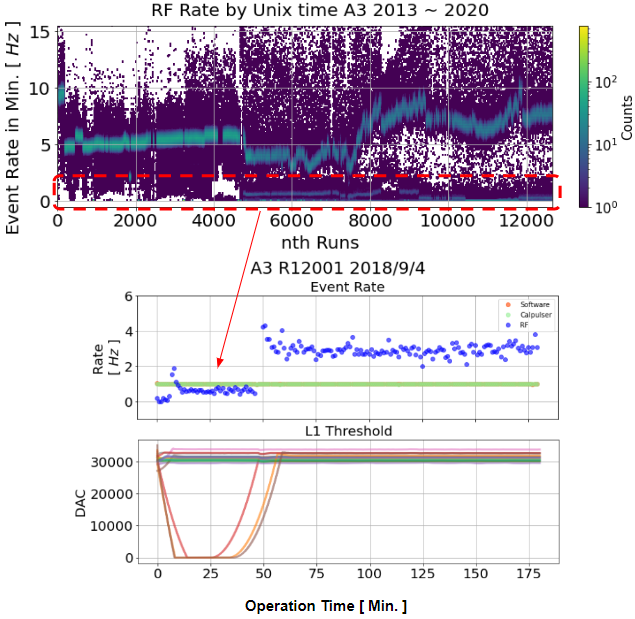
Fig. 38 top: RF event rate of all runs, middle: event rate of A2 Run12001, down: L1 threshold of A2 Run12001
L1 rate
Number of triggered events are regulated by so called dynamic threshold system
DAC value from comparator is constantly changing to keep goal of L1 rate
DAC is updated every 2 second based on data
how many time ADC value of event is bigger than DAC
It called the servo goal
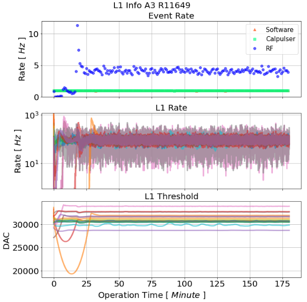
Fig. 39 Event rate, L1 rate and L1 threshold of A3 Run11649
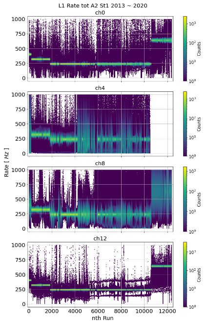
Fig. 40 L1 Rate of all data (2013 ~2022). Alignment of 1d histogram of L1 rate. Majority of run/channel is following the servo goal. But Some channels fluctuation is too big
Attempt to isolating stabilization period
Tried to isolate the period in two way
Calculate mean of L1 rate in each minute and compare with L1 goal
Calculate standard deviation of L1 rate in each minute from L1 goal
Run by run or certain time period are showing completely different rate behavior
Couldn’t set the global cut value for isolating beginning of period…
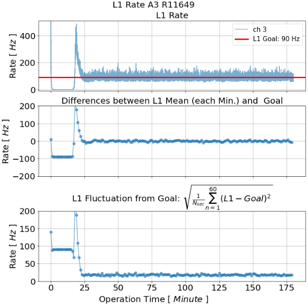
Fig. 41 L1 rate with servo goal
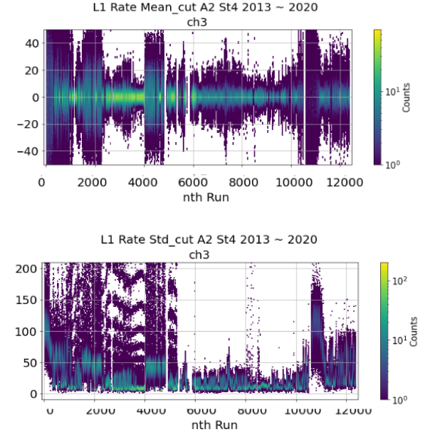
Fig. 42 mean and std of L1 rate of all runs
Simple approach for the L1 cut
Locating ‘stabilized’ period on each run by utilizing shape of L1 rate
smoothing out L1 rate fluctuation by averaging in certain time period (1 min or 10 sec)
set the cut when smoothing value is passed L1 goal value
Tried several different method
Ultimatly decied to use 10 second mean without error value
After 10 second mean, find the point smoothed line is crossed with servo goal value (1st Min from 1st Max point)
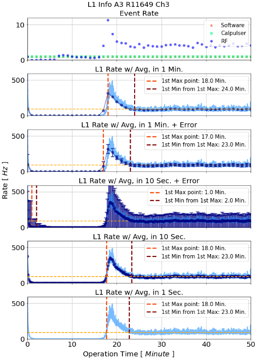
Fig. 43 Several different methods to find the flow of L1 rate
L1 cut results in event rate
2d histogram (time vs rate) of stacked RF event rate in different stage
Quality cut is all the hardware cut i developed
Looks like all the early value is nicely cut it out
But it removed 15 % of live time
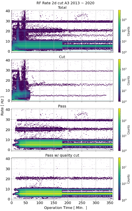
Fig. 44 2d histogram (time vs rate) of stacked RF event rate in different stage
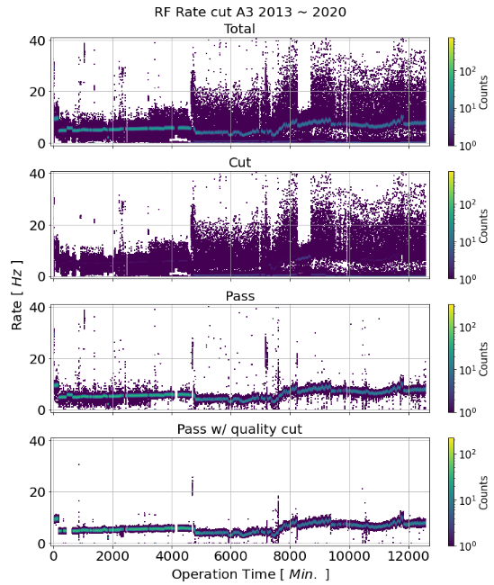
Fig. 45 2d histogram (run vs rate) of stacked RF event rate in different stage
L1 cut results in Cmax and Mmax
Distribution show events that flagged by L1 cut is located in the center of the thermal noise distribution
Since I’m not really seeing bad event from L1 cut results, I decided to exclude the L1 cut from 1st data cleaning
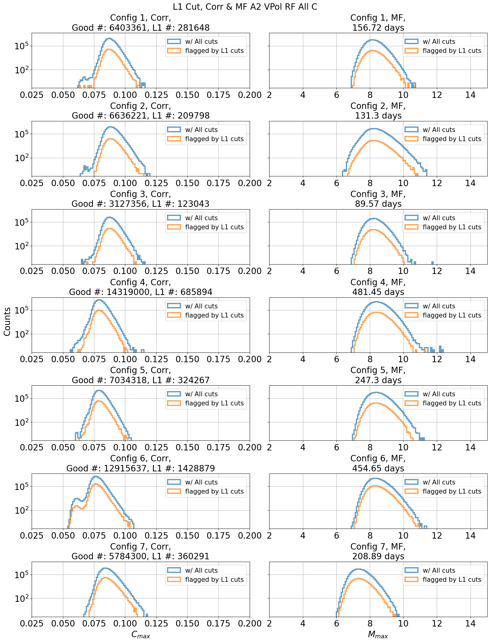
Fig. 46 A2 VPol Left: distribution in interferometry parameter. Right: distribution in matched filter parameter
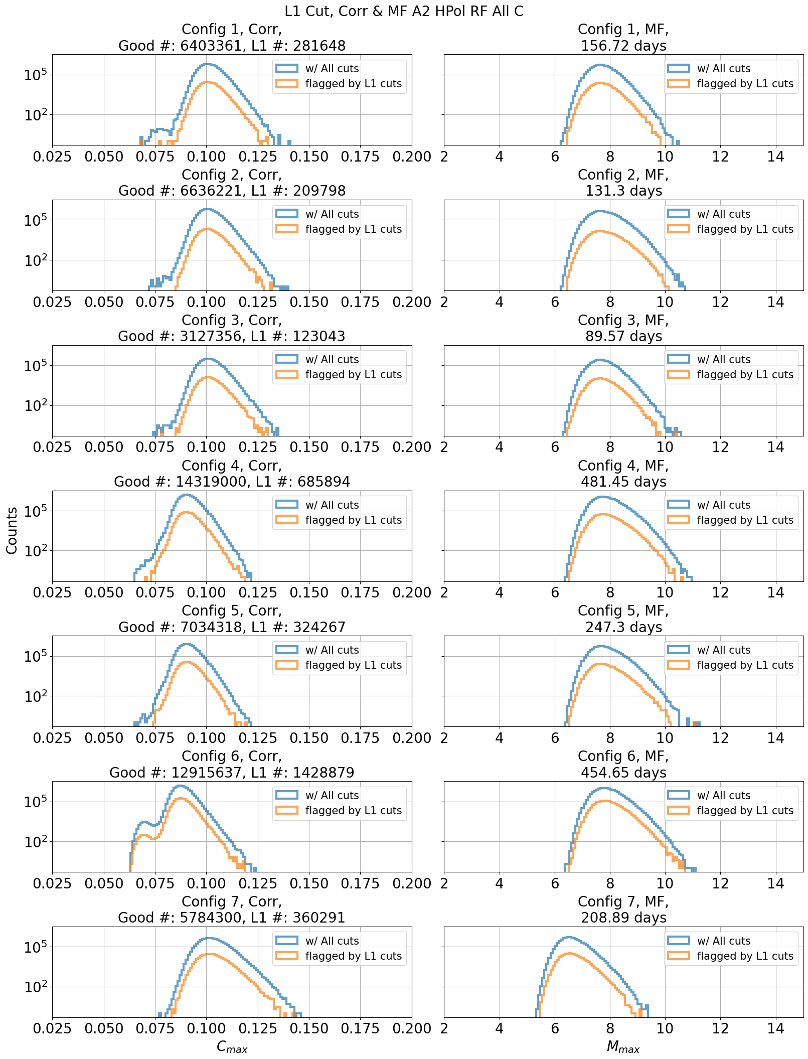
Fig. 47 A2 HPol
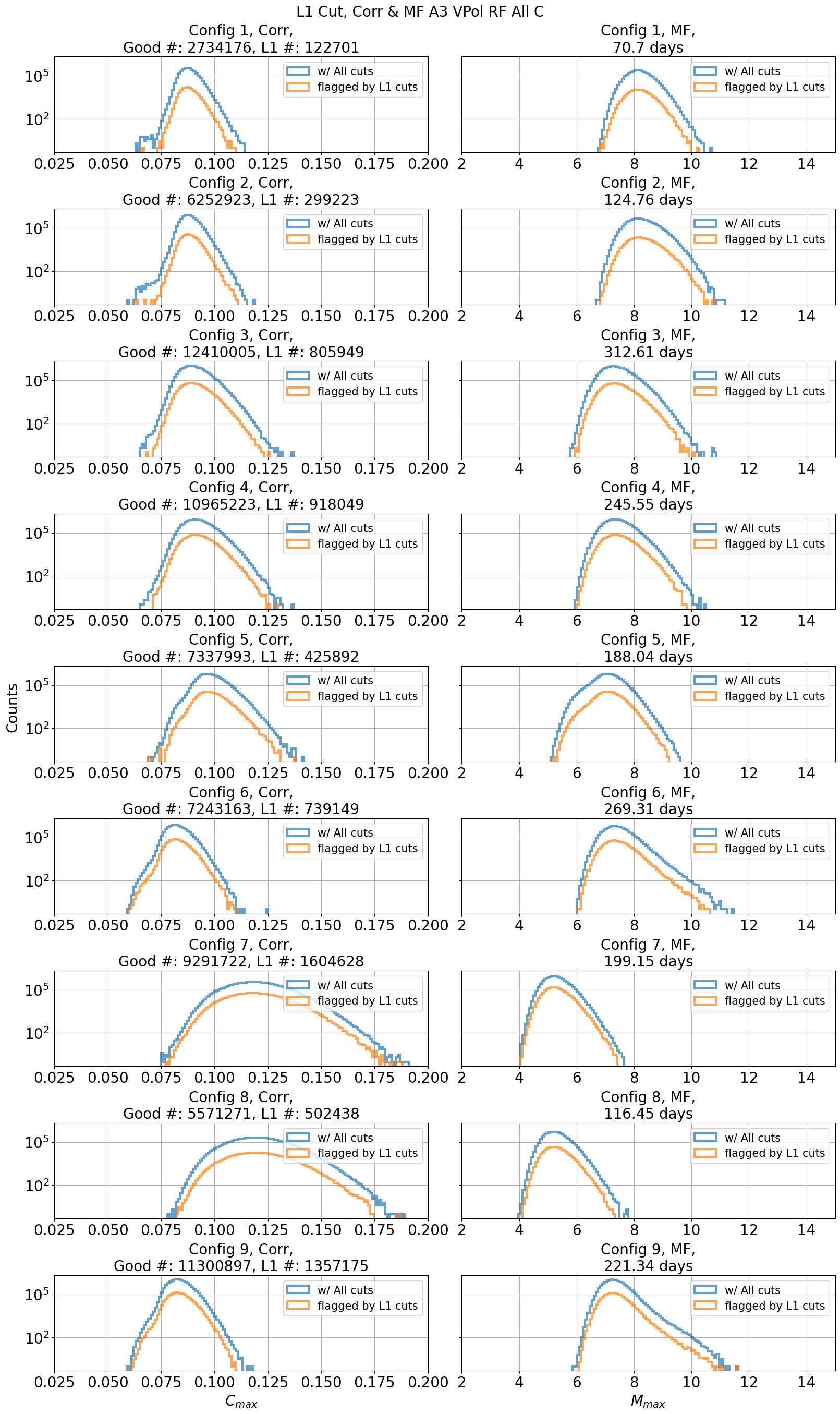
Fig. 48 A3 VPol
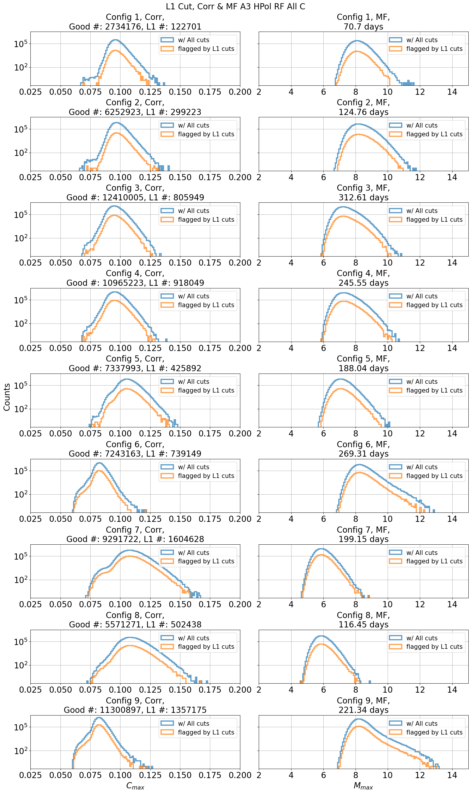
Fig. 49 A3 HPol