PISA Example Using Public IceCube Data
This analysis is a close variant of what is published in [1], and referred to as Sample B in [2] and [3]. The set of systematic uncertainties is slightly reduced and results will be close to, but not identical to the published numbers.
References:
[1] “Measurement of Atmospheric Neutrino Oscillations at 6-56 GeV with IceCube DeepCore,” IceCube Collaboration: M. G. Aartsen et al., Physical Review Letters 120, 071801 (2018). DOI: 10.1103/PhysRevLett.120.071801
[2] “Measurement of Atmospheric Tau Neutrino Appearance with IceCube DeepCore,” IceCube Collaboration: M. G. Aartsen et al., Phys. Rev. D99.3(2019), p. 032007. DOI: 10.1103/PhysRevD.99.032007
[3] “Probing the Neutrino Mass Ordering with Atmospheric Neutrinos from Three Years of IceCube DeepCore Data,” IceCube Collaboration: M.G. Aartsen et al., Feb 20, 2019, preprint: arXiv:1902.07771
Dataset must be obtained from https://icecube.wisc.edu/science/data/highstats_nuosc_3y
Setup
Usually you would need to export the location of the data, and the config files to PISA_RESOURCES. For this example however, the data is inside our package.
import numpy as np
from uncertainties import unumpy as unp
import matplotlib.pyplot as plt
import copy
import pisa
from pisa.core.distribution_maker import DistributionMaker
from pisa.core.pipeline import Pipeline
from pisa.analysis.analysis import Analysis
from pisa import FTYPE, ureg
Model
We can now instantiate the model (given our configs) that we later fit to data. This now containes two Pipelines in a DistributionMaker, one for our neutrinos, and one for the background muons.
model = DistributionMaker(["settings/pipeline/IceCube_3y_neutrinos.cfg", "settings/pipeline/IceCube_3y_muons.cfg"])
# this just turns on profiling
model.profile = True
model
| pipeline number | name | detector name | output_binning | output_key | profile |
|---|---|---|---|---|---|
| 0 | neutrinos | "dragon_datarelease": 8 (reco_energy) x 8 (reco_coszen) x 2 (pid) | ('weights', 'errors') | True | |
| 1 | muons | "dragon_datarelease": 8 (reco_energy) x 8 (reco_coszen) x 2 (pid) | ('weights', 'errors') | True |
Our model has a number of free parameters, that will be used in our fit to the data
model.params.free
| name | value | nominal_value | range | prior | units | is_fixed |
|---|---|---|---|---|---|---|
| nue_numu_ratio | 1 | 1 | [0.5, 1.5] | +/- 0.05 | dimensionless | False |
| Barr_uphor_ratio | 0 | 0 | [-3.0, 3.0] | +/- 1.0 | dimensionless | False |
| Barr_nu_nubar_ratio | 0 | 0 | [-3.0, 3.0] | +/- 1.0 | dimensionless | False |
| delta_index | 0 | 0 | [-0.5, 0.5] | +/- 0.1 | dimensionless | False |
| theta13 | 8.5 | 8.5 | [7.85, 9.1] | +/- 0.205 | degree | False |
| theta23 | 42.3 | 42.3 | [31, 59] | uniform | degree | False |
| deltam31 | 0.002457 | 0.002457 | [0.001, 0.007] | uniform | electron_volt ** 2 | False |
| aeff_scale | 1 | 1 | [0.0, 3.0] | uniform | dimensionless | False |
| nutau_norm | 1 | 1 | [-1.0, 8.5] | uniform | dimensionless | False |
| nu_nc_norm | 1 | 1 | [0.5, 1.5] | +/- 0.2 | dimensionless | False |
| opt_eff_overall | 1 | 1 | [0.8, 1.2] | +/- 0.1 | dimensionless | False |
| opt_eff_lateral | 25 | 25 | [5, 50] | +/- 10.0 | dimensionless | False |
| opt_eff_headon | 0 | 0 | [-5.0, 2.0] | uniform | dimensionless | False |
| ice_scattering | 0 | 0 | [-15, 15] | +/- 10.0 | dimensionless | False |
| ice_absorption | 0 | 0 | [-15, 15] | +/- 10.0 | dimensionless | False |
| atm_muon_scale | 1 | 1 | [0.0, 5.0] | uniform | dimensionless | False |
The two pipelines are quite different, with most complexity in the neutrino pipeline, that has several Stages and free parameters:
model.pipelines[0]
| stage number | name | calc_mode | apply_mode | has setup | has compute | has apply | # fixed params | # free params |
|---|---|---|---|---|---|---|---|---|
| 0 | csv_loader | events | events | True | False | True | 0 | 0 |
| 1 | honda_ip | "true_allsky_fine": 200 (true_energy) x 200 (true_coszen) | events | True | True | False | 1 | 0 |
| 2 | barr_simple | "true_allsky_fine": 200 (true_energy) x 200 (true_coszen) | events | True | True | False | 1 | 4 |
| 3 | prob3 | "true_allsky_fine": 200 (true_energy) x 200 (true_coszen) | events | True | True | True | 9 | 3 |
| 4 | aeff | events | events | False | False | True | 2 | 3 |
| 5 | hist | events | "dragon_datarelease": 8 (reco_energy) x 8 (reco_coszen) x 2 (pid) | True | False | True | 0 | 0 |
| 6 | hypersurfaces | "dragon_datarelease": 8 (reco_energy) x 8 (reco_coszen) x 2 (pid) | "dragon_datarelease": 8 (reco_energy) x 8 (reco_coszen) x 2 (pid) | True | True | True | 0 | 5 |
model.pipelines[0].stages[2].params
| name | value | nominal_value | range | prior | units | is_fixed |
|---|---|---|---|---|---|---|
| nu_nubar_ratio | 1 | 1 | [0.7, 1.3] | +/- 0.1 | 1 | True |
| nue_numu_ratio | 1 | 1 | [0.5, 1.5] | +/- 0.05 | 1 | False |
| Barr_uphor_ratio | 0 | 0 | [-3.0, 3.0] | +/- 1.0 | 1 | False |
| Barr_nu_nubar_ratio | 0 | 0 | [-3.0, 3.0] | +/- 1.0 | 1 | False |
| delta_index | 0 | 0 | [-0.5, 0.5] | +/- 0.1 | 1 | False |
While the muon pipleine is rather simple
model.pipelines[1]
| stage number | name | calc_mode | apply_mode | has setup | has compute | has apply | # fixed params | # free params |
|---|---|---|---|---|---|---|---|---|
| 0 | csv_icc_hist | "dragon_datarelease": 8 (reco_energy) x 8 (reco_coszen) x 2 (pid) | "dragon_datarelease": 8 (reco_energy) x 8 (reco_coszen) x 2 (pid) | True | False | True | 0 | 1 |
Retrieve Outputs
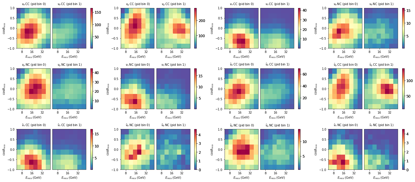
We can get individual outputs from just a pipleine like so. This fetches outputs from the neutrino pipleine, which are 12 maps.
maps = model.pipelines[0].get_outputs()
maps.names
['nue_cc',
 'numu_cc',
 'nutau_cc',
 'nue_nc',
 'numu_nc',
 'nutau_nc',
 'nuebar_cc',
 'numubar_cc',
 'nutaubar_cc',
 'nuebar_nc',
 'numubar_nc',
 'nutaubar_nc']
fig, axes = plt.subplots(3,4, figsize=(24,10))
plt.subplots_adjust(hspace=0.5)
axes = axes.flatten()

for m, ax in zip(maps, axes):
    m.plot(ax=ax)
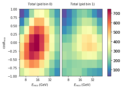
If we are interested in just the total expecatation from the full model (all neutrinos + muons), we can do the following:
model.get_outputs(return_sum=True).plot()
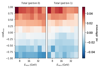
Diff plots
Let’s explore how a change in one of our nuisance parameters affects the expected counts per bin. Here we choose a hole ice parameter and move it a smidge.
# reset all free parameters to put them back to nominal values
model.reset_free()
nominal = model.get_outputs(return_sum=True)

# shift one parameter
model.params.opt_eff_lateral.value = 20
sys = model.get_outputs(return_sum=True)
((nominal[0] - sys[0])/nominal[0]).plot(symm=True, clabel="rel. difference")
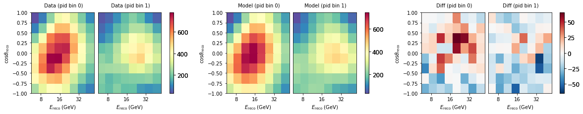
Get Data
We can load the real observed data too. This is a Pipeline with no free parameters, as the data is of course fixed. NB: When developping a new analysis you will not be allowed to look at the data as we do here before the box opening (c.f. blindness).
# real data
data_maker = Pipeline("settings/pipeline/IceCube_3y_data.cfg")
data = data_maker.get_outputs()
data_maker
| stage number | name | calc_mode | apply_mode | has setup | has compute | has apply | # fixed params | # free params |
|---|---|---|---|---|---|---|---|---|
| 0 | csv_data_hist | events | "dragon_datarelease": 8 (reco_energy) x 8 (reco_coszen) x 2 (pid) | True | False | False | 0 | 0 |
fig, ax = plt.subplots(1, 3, figsize=(20, 3))

model.reset_free()
nominal = model.get_outputs(return_sum=True)

data.plot(ax=ax[0], title="Data")
nominal.plot(ax=ax[1], title="Model")
(data - nominal).plot(ax=ax[2], symm=True, title="Diff")
Fitting
For fitting we need to configure a minimizer, several standard cfgs are available, but you can also define your own.
For the fit we need to choose a metric, and by default, theta23 octants, which are quasi degenerate, are fit seperately, which means two fits are run.
minimizer_cfg = pisa.utils.fileio.from_file('settings/minimizer/slsqp_ftol1e-6_eps1e-4_maxiter1000.json')
ana = Analysis()
%%time
result = ana.fit_hypo(
         data,
         model,
         metric='mod_chi2',
         minimizer_settings=minimizer_cfg,
         fit_octants_separately=True,
        )
[ WARNING] Minimizer slsqp requires artificial boundaries SMALLER than the user-specified boundaries (so that numerical gradients do not exceed the user-specified boundaries).
                                                                                        (deg)        (deg)       (eV**2)
 iter   funcalls    mod_chi2   | nue_numu_rat Barr_uphor_r Barr_nu_nuba delta_index    theta13      theta23      deltam31    aeff_scale   nutau_norm   nu_nc_norm  opt_eff_over opt_eff_late opt_eff_head ice_scatteri ice_absorpti atm_muon_sca
------ ---------- ------------ + ------------ ------------ ------------ ------------ ------------ ------------ ------------ ------------ ------------ ------------ ------------ ------------ ------------ ------------ ------------ ------------
  0        6       1.75086e+02 |  1.00000e+00  0.00000e+00  0.00000e+00  0.00000e+00  8.50013e+00  4.23000e+01  2.45700e-03  1.00000e+00  1.00000e+00  1.00000e+00  1.00000e+00  2.50000e+01  0.00000e+00  0.00000e+00  0.00000e+00  1.00000e+00
---------------------------------------------------------------------------
KeyboardInterrupt                         Traceback (most recent call last)
<timed exec> in <module>

~/pisa/pisa/analysis/analysis.py in fit_hypo(self, data_dist, hypo_maker, metric, minimizer_settings, hypo_param_selections, reset_free, check_octant, fit_octants_separately, check_ordering, other_metrics, blind, pprint, external_priors_penalty)
    511                 pprint=pprint,
    512                 blind=blind,
--> 513                 external_priors_penalty=external_priors_penalty
    514             )
    515

~/pisa/pisa/analysis/analysis.py in fit_hypo_inner(self, data_dist, hypo_maker, metric, minimizer_settings, other_metrics, pprint, blind, external_priors_penalty)
    776             method=minimizer_settings['method']['value'],
    777             options=minimizer_settings['options']['value'],
--> 778             callback=self._minimizer_callback
    779         )
    780         end_t = time.time()

~/.local/lib/python3.7/site-packages/scipy/optimize/_minimize.py in minimize(fun, x0, args, method, jac, hess, hessp, bounds, constraints, tol, callback, options)
    616     elif meth == 'slsqp':
    617         return _minimize_slsqp(fun, x0, args, jac, bounds,
--> 618                                constraints, callback=callback, **options)
    619     elif meth == 'trust-constr':
    620         return _minimize_trustregion_constr(fun, x0, args, jac, hess, hessp,

~/.local/lib/python3.7/site-packages/scipy/optimize/slsqp.py in _minimize_slsqp(func, x0, args, jac, bounds, constraints, maxiter, ftol, iprint, disp, eps, callback, **unknown_options)
    421             # Compute the derivatives of the objective function
    422             # For some reason SLSQP wants g dimensioned to n+1
--> 423             g = append(fprime(x), 0.0)
    424
    425             # Compute the normals of the constraints

~/.local/lib/python3.7/site-packages/scipy/optimize/optimize.py in function_wrapper(*wrapper_args)
    325     def function_wrapper(*wrapper_args):
    326         ncalls[0] += 1
--> 327         return function(*(wrapper_args + args))
    328
    329     return ncalls, function_wrapper

~/.local/lib/python3.7/site-packages/scipy/optimize/slsqp.py in approx_jacobian(x, func, epsilon, *args)
     61     for i in range(len(x0)):
     62         dx[i] = epsilon
---> 63         jac[i] = (func(*((x0+dx,)+args)) - f0)/epsilon
     64         dx[i] = 0.0
     65

~/.local/lib/python3.7/site-packages/scipy/optimize/optimize.py in function_wrapper(*wrapper_args)
    325     def function_wrapper(*wrapper_args):
    326         ncalls[0] += 1
--> 327         return function(*(wrapper_args + args))
    328
    329     return ncalls, function_wrapper

~/pisa/pisa/analysis/analysis.py in _minimizer_callable(self, scaled_param_vals, hypo_maker, data_dist, metric, counter, fit_history, pprint, blind, external_priors_penalty)
   1113                 metric_kwargs = {'empty_bins':hypo_maker.empty_bin_indices}
   1114             else:
-> 1115                 hypo_asimov_dist = hypo_maker.get_outputs(return_sum=True)
   1116                 if isinstance(hypo_asimov_dist, OrderedDict):
   1117                     hypo_asimov_dist = hypo_asimov_dist['weights']

~/pisa/pisa/core/distribution_maker.py in get_outputs(self, return_sum, sum_map_name, sum_map_tex_name, **kwargs)
    250
    251         outputs = [pipeline.get_outputs(**kwargs) for pipeline in self] # pylint: disable=redefined-outer-name
--> 252
    253         if return_sum:
    254

~/pisa/pisa/core/distribution_maker.py in <listcomp>(.0)
    250
    251         outputs = [pipeline.get_outputs(**kwargs) for pipeline in self] # pylint: disable=redefined-outer-name
--> 252
    253         if return_sum:
    254

~/pisa/pisa/core/pipeline.py in get_outputs(self, output_binning, output_key)
    305
    306         self.run()
--> 307
    308         if output_binning is None:
    309             output_binning = self.output_binning

~/pisa/pisa/core/pipeline.py in run(self)
    329         for stage in self.stages:
    330             logging.debug(f"Working on stage {stage.stage_name}.{stage.service_name}")
--> 331             stage.run()
    332
    333     def setup(self):

~/pisa/pisa/core/stage.py in run(self)
    368
    369     def run(self):
--> 370         self.compute()
    371         self.apply()
    372         return None

~/pisa/pisa/core/stage.py in compute(self)
    338         if self.profile:
    339             start_t = time()
--> 340             self.compute_function()
    341             end_t = time()
    342             self.calc_times.append(end_t - start_t)

~/pisa/pisa/stages/osc/prob3.py in compute_function(self)
    316                             container['densities'],
    317                             container['distances'],
--> 318                             out=container['probability'],
    319                            )
    320             container.mark_changed('probability')

~/pisa/pisa/stages/osc/prob3.py in calc_probs(self, nubar, e_array, rho_array, len_array, out)
    231                         rho_array,
    232                         len_array,
--> 233                         out=out
    234                        )
    235

KeyboardInterrupt:
Here we can view the bestfit parameters - the result of our fit.
We have run two fits (separately for each theta23 octant), and the best result is stored in results[0] (both fits are also available under results[1])
bestfit_params = result[0]['params'].free
bestfit_params
| name | value | nominal_value | range | prior | units | is_fixed |
|---|---|---|---|---|---|---|
| nue_numu_ratio | 1.03304 | 1 | [0.5, 1.5] | +/- 0.05 | dimensionless | False |
| Barr_uphor_ratio | -0.313404 | 0 | [-3.0, 3.0] | +/- 1.0 | dimensionless | False |
| Barr_nu_nubar_ratio | -0.0200293 | 0 | [-3.0, 3.0] | +/- 1.0 | dimensionless | False |
| delta_index | -0.0106011 | 0 | [-0.5, 0.5] | +/- 0.1 | dimensionless | False |
| theta13 | 8.50992 | 8.5 | [7.85, 9.1] | +/- 0.205 | degree | False |
| theta23 | 46.2525 | 42.3 | [31, 59] | uniform | degree | False |
| deltam31 | 0.00242605 | 0.002457 | [0.001, 0.007] | uniform | electron_volt ** 2 | False |
| aeff_scale | 0.934868 | 1 | [0.0, 3.0] | uniform | dimensionless | False |
| nutau_norm | 0.610718 | 1 | [-1.0, 8.5] | uniform | dimensionless | False |
| nu_nc_norm | 1.26342 | 1 | [0.5, 1.5] | +/- 0.2 | dimensionless | False |
| opt_eff_overall | 1.05348 | 1 | [0.8, 1.2] | +/- 0.1 | dimensionless | False |
| opt_eff_lateral | 22.0081 | 25 | [5, 50] | +/- 10.0 | dimensionless | False |
| opt_eff_headon | -1.32275 | 0 | [-5.0, 2.0] | uniform | dimensionless | False |
| ice_scattering | -2.87791 | 0 | [-15, 15] | +/- 10.0 | dimensionless | False |
| ice_absorption | 1.76103 | 0 | [-15, 15] | +/- 10.0 | dimensionless | False |
| atm_muon_scale | 0.931489 | 1 | [0.0, 5.0] | uniform | dimensionless | False |
# update the model with the bestfit (make a copy here, because we don't want our bestfit params to be affected (NB: stuff is passed by reference in python))
model.update_params(copy.deepcopy(bestfit_params))
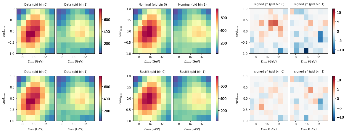
Let’s see how good that fit looks like. We here construct signed mod_chi2 maps by hand. You can see that after the fit, it improved considerably, and the distribution of chi2 values is now more uniform - not much features can be seen anymore.
fig, ax = plt.subplots(2, 3, figsize=(20, 7))
plt.subplots_adjust(hspace=0.5)

bestfit = model.get_outputs(return_sum=True)

data.plot(ax=ax[0,0], title="Data")
nominal.plot(ax=ax[0,1], title="Nominal")
diff = data - nominal
(abs(diff)*diff/(nominal + unp.std_devs(nominal.hist['total']))).plot(ax=ax[0,2], symm=True, title=r"signed $\chi^2$", vmin=-12, vmax=12)

data.plot(ax=ax[1,0], title="Data")
bestfit.plot(ax=ax[1,1], title="Bestfit")
diff = data - bestfit
(abs(diff)*diff/(bestfit + unp.std_devs(bestfit.hist['total']))).plot(ax=ax[1,2], symm=True, title=r"signed $\chi^2$", vmin=-12, vmax=12)
When checking the chi2 value from the fitted model, you maybe see that it is around 113, while in the minimizer loop we saw it converged to 116. It is important to keep in mind that in the fit we had extended the metric with prior penalty terms. When we add those back we get the identical number as reported in the fit.
print(data.metric_total(nominal, 'mod_chi2'))
print(data.metric_total(bestfit, 'mod_chi2'))
175.08610154304426
113.03553972952989
Evaluating other metrics just for fun:
for metric in pisa.utils.stats.ALL_METRICS:
    try:
        print('%s = %.3f'%(metric,data.metric_total(bestfit, metric)))
    except:
        print('%s failed'%metric)
llh = -64.972
conv_llh = -57.326
barlow_llh = -1147.290
mcllh_mean = -541.333
mcllh_eff = -541.486
generalized_poisson_llh failed
chi2 = 128.476
mod_chi2 = 113.036
Adding prior penalty terms
model.update_params(copy.deepcopy(bestfit_params))
data.metric_total(bestfit, 'mod_chi2') + model.params.priors_penalty('mod_chi2')
115.8086745310561
result[0]['metric_val']
115.8086745310561
Storing the results to a file
Since the fit took a while, it might be useful to store the results to a file. (NB: in this example we use a temp file, but in real life you would of course just use a real pathname instead!)
import tempfile
temp = tempfile.NamedTemporaryFile(suffix='.json')
pisa.utils.fileio.to_file(result, temp.name)
[ WARNING] Overwriting file at '/tmp/tmp04yxkl60.json'
To reload, we can read the file. But to get PISA objects back, they need to instantiated
result_reload = pisa.utils.fileio.from_file(temp.name)
bestfit_params = pisa.core.ParamSet(result_reload[0]['params']).free
bestfit_params
temp.close()
Profiling
To understand what parts of the model were executed how many times, and how long it took, the profiling can help:
model.pipelines[0].report_profile()
data csv_loader
- setup:  Total time 0.00000 s, n calls: 0, time/call: 0.00000 s
- calc:   Total time 0.00000 s, n calls: 0, time/call: 0.00000 s
- apply:  Total time 1.34596 s, n calls: 817, time/call: 0.00165 s
flux honda_ip
- setup:  Total time 0.00000 s, n calls: 0, time/call: 0.00000 s
- calc:   Total time 25.08353 s, n calls: 1, time/call: 25.08353 s
- apply:  Total time 0.00072 s, n calls: 817, time/call: 0.00000 s
flux barr_simple
- setup:  Total time 0.00000 s, n calls: 0, time/call: 0.00000 s
- calc:   Total time 118.13966 s, n calls: 330, time/call: 0.35800 s
- apply:  Total time 0.00091 s, n calls: 817, time/call: 0.00000 s
osc prob3
- setup:  Total time 0.00000 s, n calls: 0, time/call: 0.00000 s
- calc:   Total time 339.71126 s, n calls: 290, time/call: 1.17142 s
- apply:  Total time 73.15262 s, n calls: 817, time/call: 0.08954 s
aeff aeff
- setup:  Total time 0.00000 s, n calls: 0, time/call: 0.00000 s
- calc:   Total time 0.00056 s, n calls: 290, time/call: 0.00000 s
- apply:  Total time 1.62155 s, n calls: 817, time/call: 0.00198 s
utils hist
- setup:  Total time 0.00000 s, n calls: 0, time/call: 0.00000 s
- calc:   Total time 0.00000 s, n calls: 0, time/call: 0.00000 s
- apply:  Total time 73.78663 s, n calls: 817, time/call: 0.09031 s
discr_sys hypersurfaces
- setup:  Total time 0.00000 s, n calls: 0, time/call: 0.00000 s
- calc:   Total time 0.27885 s, n calls: 372, time/call: 0.00075 s
- apply:  Total time 0.44868 s, n calls: 817, time/call: 0.00055 s