John Kelley, UW-Madison, May 2005
![]()
To estimate the background, we first define an on-source and off-source region. The on-source region is defined as a region of the sky within a certain number of degrees (say, 5) within the galactic equator, that is, (-5 < galactic latitude < 5). This traces a band across the sky, centered around (b=0).
The background is estimated from the off-source region, but because the background rate is dependent on the declination, we use 5-degree slices of declination, starting from the horizon, to estimate the background in the on-source region at that declination:
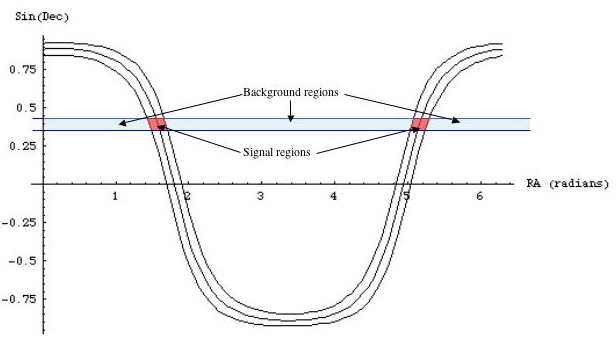
Figure 4.1: On-source and off-source regions used for background estimation.
Specifically, the background estimate in the on-source region around declination D, (D-2.5 < declination < D+2.5) is given by the count in the off-source region scaled by the ratio of the solid angles. Note that the regions do not have simple shapes, so the solid angle is determined by numerical integration of the function defining the on-source band. This calculation has been checked by comparing the estimated background with the "signal" from the scrambled data, as well as by comparing with published solid angles.
The sensitivity can be estimated using the standard model rejection factor prescription using the total number of signal events in the on-source region. The line source signal is convolved with the angular response of the detector, which results in the line spread function around the plane:
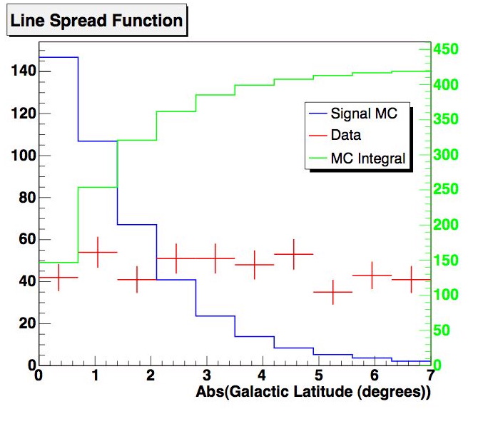
Figure 4.2: Line spread function of signal MC (high signal normalization).
This plot illustrates that the sensitivity can be optimized by an appropriate choice of the on-source region width. Optimizing the model rejection factor as a function of this width results in an optimimal region 4 degrees wide (-2 < galactic latitude < 2):
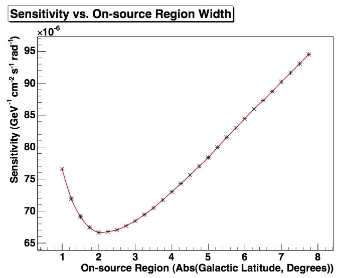
Figure 4.3: Sensitivity to a line source (spectral index -2.7) as a function of on-source region width.
Admittedly, this optimization is a bit artificial, since the signal hypothesis is artificially narrow (a line). Nevertheless, we can still use this procedure as a method to determine the on-source region to use. This table illustrates how this final angular cut affects the passing rates of signal and background:
Cut level |
Signal MC, high normalization |
Atmospheric MC |
Data (scrambled) |
| Level 4 + Zenith[7]>90 | 895.6 |
9431 |
5.677M |
| Final point source cuts | 422.8 |
3196 |
3329 |
| Galactic angular cut (abs(Bb[7]) < 2.0) | 311.8 |
121.2 |
133 |
Table 4.1: Passing rates for scrambled data and Monte Carlo (below horizon), including final optimized angular cut.
The estimated background in the +/-2 degree on-source region is 129.4, which is close to the scrambled-data value of 133.
The optimal MRF results in a sensitivity of the following, for a spectral index of -2.7 :
![]()
Note that the units on this sensitivity are per radian, not per steradian, since the signal is a line flux. Furthermore, no adjustments have been made to this sensitivity (or any following sensitivity) for oscillations.
We would like to investigate how this sensitivity to a line flux can be used to estimate the sensitivity to other signal hypotheses (without regenerating the signal Monte Carlo). The key to this method is to calculate a normalization of the new signal flux hypothesis which would give the same number of signal events in the on-source region as the line flux sensitivity, with some important approximations.
The simplest case is a "diffuse" step-function flux around the galactic equator (diffuse in the sense that it's now truly a flux per steradian). Our sensitivity to that flux would be that which gives us the same number of events in the on-source region. We approximate that in the narrow on-source region, the step-function flux convolved with the detector response is still a step function (not exactly true, because we don't take into account the variation in response for slightly different zenith angles in the on-source window).
Thus we can write:
![]()
where the quantity in parenthesis is the linear flux integrated over galactic longitude (pi radians in one hemisphere), with an efficiency factor eta of 0.74, the amount of signal in the on-source region of +/- two degrees. The solid angle omega is the solid angle (in equatorial coordinates!) of the on-source region (0.22 sr).
This results in a sensitivity to a diffuse flux in the on-source region of the following, for a spectral index of -2.7:
![]()
The following figure shows this sensitivity on the Learned and Mannheim plot (dotted red line). The horizontal range of the sensitivity shown is the energy range covering 5% to 95% of the signal, after the final galactic angular cut.
Figure 4.4: Sensitivity of this analysis (red dotted line)
to a diffuse flux in a band +/-2 degrees around the galactic equator (spectral
index -2.7).
Energy range covered is the 5-95% region of the signal spectrum.
The sensitivity to a line source has also been computed for spectral indices as hard as -2.4, and as soft as -2.9. The optimal on-source region is not affected by spectral index and is +/- two degrees in each case:
Spectral Index |
Sensitivity (per radian) |
Sensivitity (per steradian) |
-2.4 |
5.4e-6 |
5.7e-5 |
-2.5 |
1.3e-5 |
1.4e-4 |
-2.6 |
3.0e-5 |
3.2e-4 |
-2.7 |
6.7e-5 |
7.1e-4 |
-2.8 |
1.4e-4 |
1.5e-3 |
-2.9 |
3.1e-4 |
3.3e-3 |
Table 4.1: Sensitivity to a line source for different spectral indices
The estimated step-function diffuse sensitivity in the optimized on-source region for three of these indices are shown in the following figure. Again, the horizontal range of the sensitivity shown is the 5% to 95% energy range of the signal Monte Carlo after all cuts, including the galactic angular cut.
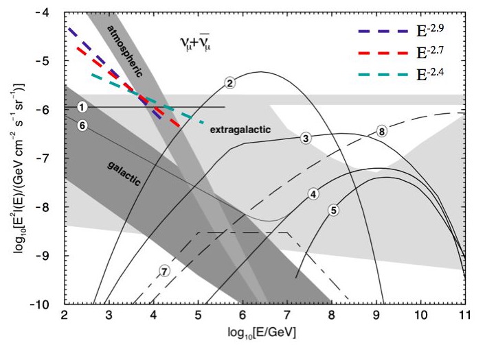
Figure 4.5: Sensitivity of this analysis (dotted lines) to
diffuse step-function fluxes with spectral indices from -2.4 to -2.9,
in a band +/-2 degrees around the galactic equator.
Energy ranges covered are the 5-95% regions of the signal spectra.
A method for estimating the sensitivity to a signal which is Gaussian in galactic latitude has also been developed. If one approximates the line spread function as Gaussian of width 1.5 degrees, then the convolution of the Gaussian LSF with a Gaussian signal will result in another Gaussian around the galactic equator as the final signal distribution:
![]()
Also, in this case, the previously introduced efficiency factor eta can be approximated in terms of an error function, for an on source region of +/-B degrees:

Using the same technique as before, we equalize the number of events in the signal region, and we find an expression for the Gaussian signal sensitivity:

Fitting the Strong et al. pi-zero distribution shown in Section 1 to a Gaussian (it's not Gaussian, the tails are too large — but it's approximately Gaussian near the equator) gives a signal with a sigma of 2.1 degrees. So we can estimate our sensitivity to a neutrino flux with the same shape, and a spectral index of -2.7, as the following, by evaluating the previous expression numerically:
![]()
As expected, this sensitivity is slightly worse than the sensitivity to a diffuse step-function in the same region. However, this on-source region was chosen to minimize the line-flux sensitivity. By considering the line-flux sensitivity as a function of the on-source region size (Figure 4.3), we can reoptimize by finding the on-source region size which minimizes the Gaussian sensitivity function above. This sensitivity as a function of the on-source region size is shown below:
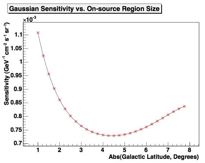
Figure 4.5: Sensitivity to Gaussian signal as a function of on-source region size.
The minimum of this curve is at a larger on-source window size of +/-4.4 degrees (8.8 degrees wide total).
This results in the following sensitivity to a Gaussian signal with spectral index -2.7 and sigma of 2.1 degrees:
![]()
This discussion was a bit abbreviated, but a more detailed derivation of the equations used can be found in the following document:
Gaussian sensitivity calculations (pdf, 70K)