Tidbits

Weighting tricks

Combining weighted simulation

dCORSIKA

There are times when it is useful to combine weighted Corsika simulation from runs with different generation spectra. Calculating the appropriate weights for combined sets turns out to be remarkably simple, provided that one understands how the weighting works. The simplest form of an importance-sampling weight (in units of 1/time) for a cosmic-ray primary of energy \(E\) is:

\[w(E) = \frac{A_{total}}{N p_{gen}(E)} \Phi_{target}(E)\]

where \(A_{total}\) is the integrated area-times-solid-angle of the sampling surface, \(N\) is the number of generated events, \(\Phi_{target}\) is flux one wishes to weight to, and \(p_{gen}\) is the probability of drawing the given \(E\) from the generation spectrum. For a power-law generation spectrum between energies \(E_0\) and \(E_1\) the generation probability is just:

\[\begin{split}p_{gen}(E,Z) = \begin{cases} \frac{E^{-\gamma}}{\int_{E_{0}}^{E_{1}} E^{-\gamma} dE} & \mbox{if } E_0 \leq E \lt E_1 \\ 0 & \mbox{otherwise } \end{cases}\end{split}\]

The extension to multiple primaries, or multiple samples with different generation spectra, is straightforward. Instead of normalizing to a single generation spectrum \(N p_{gen}(E)\), one normalizes to a combined distribution that is a sum of the generation spectra, weighted by the number of entries drawn from each:

\[N_{total} \hat{p}_{gen}(E,Z) = \sum_i N_{Z,i} p_{gen,i}(E,Z)\]

So the weight for events from the combined sample is:

\[\hat{w}(E,Z) = \frac{A_{total}}{\sum_i N_{Z,i} p_{gen,i}(E,Z)} \Phi_{target}(E,Z)\]

The only technical difference to the single-set case is that the combined generation probability \(\hat{p}_{gen}(E,Z)\) is defined piecewise.

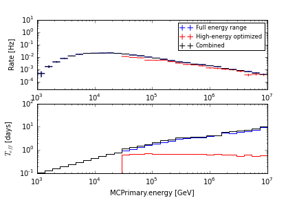
A demonstration of combined weights for different generation spectra. The “Full energy range” sample was generated from an \(E^{-2}\) spectrum across the full range of energies that trigger IceCube, while the “High-energy optimized” sample was generated from a more natural \(E^{-2.6}\) spectrum with a high energy treshold. While the combined histogram closely follows that of the (larger) full-range sample, the effective livetime plot shows how the addition of the high-threshold sample begins to reduce the variance of the combined sample above its threshold.

Math to CorsikaWeightMap translation guide

Expression	Key in CorsikaWeightMap
\(A_{total}\)	AreaSum
\(r_{gen}\)	CylinderRadius
\(l_{gen}\)	CylinderLength
\(-\gamma\)	PrimarySpectralIndex
\(E_0\)	EnergyPrimaryMin
\(E_1\)	EnergyPrimaryMax
\(\int_{E_{0}}^{E_{1}} E^{-\gamma} dE\)	FluxSum
\(N_{i,Z}\)	NEvents (times NFiles)

Aside: unweighted Hörandel

In RANPRI=2 mode, dCORSIKA generates primaries through iron from the parametrization of Hörandel (2003). Just as with power-law generated spectra, these sets can be combined with weighted sets given knowledge of \(N p_{gen}(E,Z)\). The generated flux is of the form:

\[\frac{d\Phi(E,Z)}{dE} = \Phi_0(Z) E^{-\gamma_Z} \left( 1 + \left(\frac{E}{E_{knee}Z}\right)^{\epsilon} \right)^{-\Delta \gamma / \epsilon}\]

The knee term makes the calculation of the normalization of the generation PDF somewhat tricky. As it turns out, the antiderivative involves a Gauss hypergeometric function:

\[\Phi(E,Z) = \Phi_0(Z) \frac{E^{1-\gamma_Z}}{1-\gamma_Z} \,_2F_1\left(\frac{\Delta \gamma}{\epsilon}, \frac{1-\gamma_Z}{\epsilon}; \frac{1-\gamma_Z}{\epsilon}+1, -\left(\frac{E_0}{E_{knee}Z}\right)^{\epsilon} \right)\]

The biasing mode of dCORSIKA (DSLOPE != 0) simply adds a constant factor to each \(\gamma_Z\); the knee simulated via acceptance-rejection sampling just as in the unbiased mode.

NeutrinoGenerator

The same trick works for neutrino-generator data, with a few names changed. Here the weight is of the form

\[w(E, \theta) = p_{int} \frac{A \Omega}{N p_{gen}(E)} \Phi_{target}(E, \theta)\]

where \(A \equiv \pi r_{gen}^2 / {\rm cm}\) is the total area of neutrino-generator’s injection surface, \(\Omega \equiv (\cos{\theta_1}-\cos{\theta_0})(\phi_1-\phi_0) / {\rm sr}\) is the solid angle over which events were generated, and \(p_{int}\) is the probability that the neutrino would have interacted at the point in the detector where it was forced to. Just as before, the weight for combined samples with different generation spectra is:

\[\hat{w}(E, \theta) = p_{int} \frac{A \Omega}{\sum_i N_{i} p_{gen,i}(E)} \Phi_{target}(E, \theta)\]

In contrast to Corsika weights, the multi-sample case for neutrino-generator data is slightly more annoying to implement, as one has to calculate \(A\), \(\Omega\), and \(\int_{E_{0}}^{E_{1}} E^{-\gamma} dE\) after the fact instread of taking the pre-packaged OneWeight.

Math to I3MCWeightDict translation guide

Expression	Key in I3MCWeightDict
\(r_{gen}\)	InjectionSurfaceR
\(l_{gen}\)	TotalDetectionLength
\(p_{int}\)	TotalInteractionProbabilityWeight
\(\gamma\)	PowerLawIndex
\(\log_{10}{E_0}\), \(\log_{10}{E_1}\)	MinEnergyLog, MaxEnergyLog
\(\theta_0\), \(\theta_1\)	MinZenith, MaxZenith
\(\phi_0\), \(\phi_1\)	MinAzimuth, MaxAzimuth
\(p_{int} \frac{A \Omega}{p_{gen}(E)}\)	OneWeight

Effective areas

Note

I know that everyone knows how to do this; this section is more for my own benefit than anyone else’s.

NeutrinoGenerator

NeutrinoGenerator’s simulation volume is a cylinder of a fixed radius \(r_{gen}\) whose length varies for each injected neutrino energy to accomodate the range of possible muons produced in the interaction. Neutrino energies are drawn from a fixed power law distribution and forced to interact at a random distance along the cylinder chosen from a uniform distribution, and the probability of that forced interaction is stored as a weight \(p_{int}\). These factors can be combined to yield the commonly-used OneWeight:

\[OneWeight = \pi r_{gen}^2 \Omega \frac{p_{int}}{N p_{gen}} \,\, {\rm cm}^2\,{\rm sr}\,{\rm GeV}\]

where energy unit comes from the fact that the generation probability is in units of 1/energy. The weights of events surviving some selection can be used to express a detection efficiency in a given neutrino energy range in units of area:

\[A_{eff} = \frac{\frac{\pi r_{gen}^2\Omega}{4\pi} \sum_i \frac{p_{int,i}}{N p_{gen,i}}}{\Delta E}\]

where \(\Delta E\) is a range of energies being summed over. If the interaction probability were exactly one, the ratio of the effective area to the injection area would simply be a measure of the cut efficiency; the interaction probability folds in the effects of the neutrino-nucleon cross-section. Intuitively, the effective area is the area of an equivalent perfectly-absorbing neutrino detector. For point-like events (starting muons, cascades), it also makes sense to define an effective volume. Instead of counting up weighted contributions to the injection area, we can instead count up weighted contributions to the simulation volume, and define:

\[V_{eff} = \frac{\frac{\pi r_{gen}^2 \Omega}{4\pi} \sum_i l_{gen,i}\frac{p_{int,i}}{N p_{gen,i}}}{\Delta E}\]

where \(l_{gen}\) length of the generation cylinder. If one wants to ignore the probability of seeing a neutrino in the first place and simply express an effective selection volume, one can omit the interaction probability to define a fiducial volume:

\[V_{fiducial} = \frac{\frac{\Omega}{4\pi} \sum_i \frac{l_{gen,i}}{N p_{gen,i}}}{\Delta E}\]

dCORSIKA

An analogous effective area can be defined for dCORSIKA simulation, with the simplification that forced interactions are unnecessary:

\[A_{eff} = \frac{\frac{A_{total}}{2\pi} \sum_i \frac{1}{N p_{gen,i}}}{\Delta E}\]