| In-Ice Cable
|
|
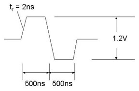
| RAP cal input pulse characteristics
|
|
| COMM ADC
|
*ADC input range (2V) divided by the differential preamp gain (5).
|
Cable Filter Design
N. Kitamura
03/26/2004
Purpose of the Cable Filter
*TBR--To Be Reviewed.
**What is considered smooth must be discussed and agreed upon.
This webpage focuses on the design and implementation of the filter. For information of the RAPcal measurements at UW-Madison, see Mark Krasberg's webpage.
Assumptions
In-Ice Cable
- Nominal length = 3.5 km
- Characteristic impedance = 145 Ohm
- Loop resistance = 44 Ohm / km
RAP cal input pulse characteristics
COMM ADC
- Sampling rate = 20 MHz
- Resolution = 10 bit
- Scale = 400mV* per 1024 counts.
*ADC input range (2V) divided by the differential preamp gain (5).
Filter Design Information
Summary: CableFltDoc.pdf
Andy Laundrie's design info for various cable length with datasheets: http://docushare.icecube.wisc.edu/docushare/dsweb/View/Collection-994
Gerber files: CableFlt2.zip
Simulated response (3.5km filter)
Ouptut DFLFILT3K5MA.pdf
Netlist DFLFILT3K5MA_NET.pdf
Schematic DFLFILT3K5MA_sch.pdf
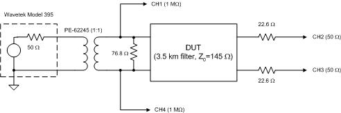
Measured response with an arbitrary waveform generator source
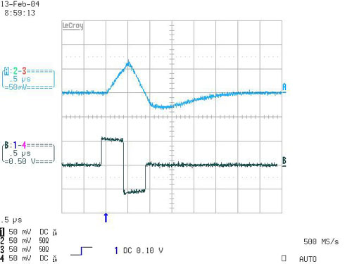 |
Setup diagram: labsetup.jpg
Numerical data:
|
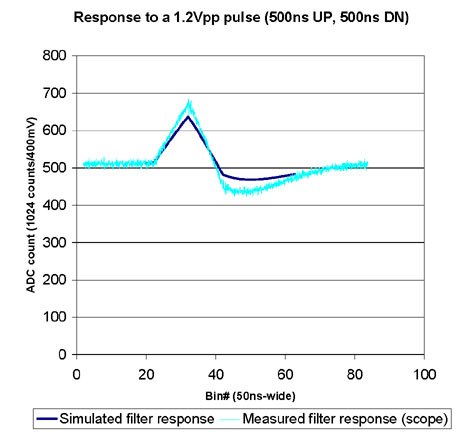
Comparison: Simulation vs Actual Response
(The curves have been manually shifted in x-direction to overlap with one another.)
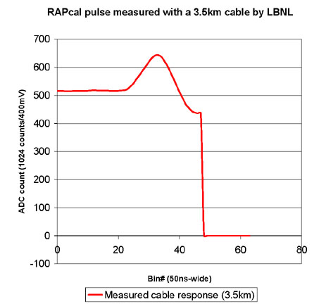
Comparison: Filtered Response vs Long Cable's Response
(The curves have been manually shifted in x-direction to overlap with one another.)
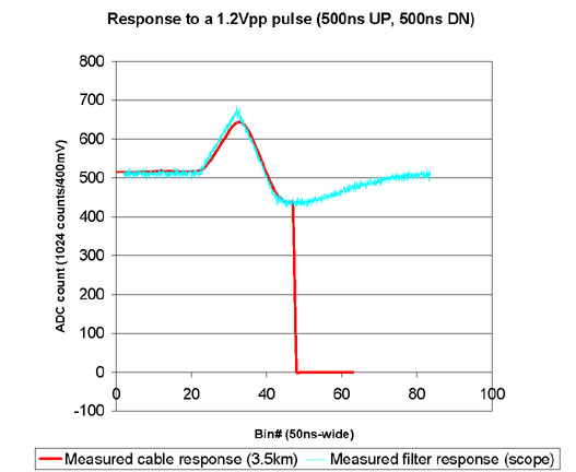
Why is the red curve smoother? ==> Because Kalle's FPGA code performs a running average over every four sampled points. See Kalle's presentation (page 17): running_ave/DOR_DOM_Comm.pdf
How the running average was applied to the scope data is shown in the mathcad document: running_ave/running_ave.pdf
If you want to run the MathCad document yourself, use the following:
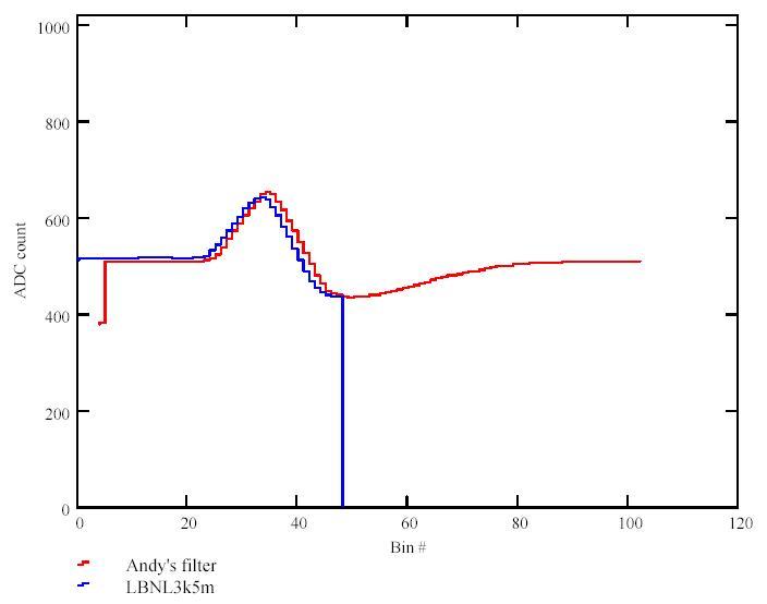
The comparison of the two curves, after applying the running average is shown below:
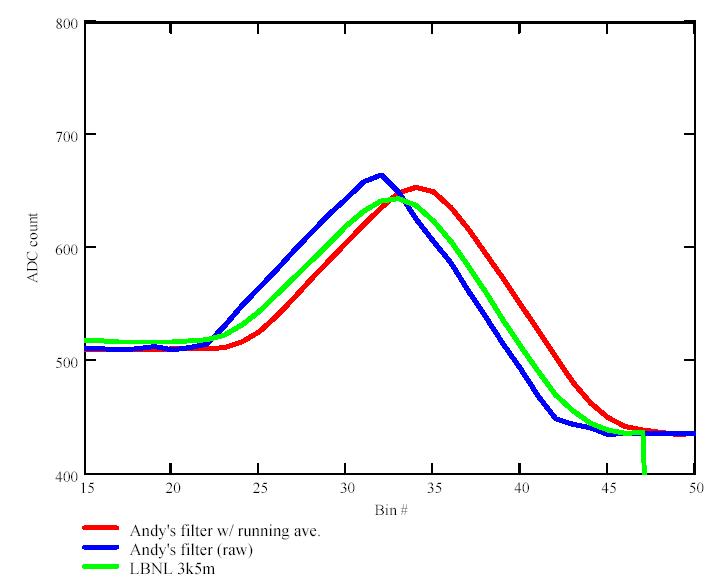
The scope measurement with and without the running average, as well as the LBNL cable data, are compared in the below (magnified view):
Finally, the red and the green are shifted relative to each other and are compared (now in physical units):
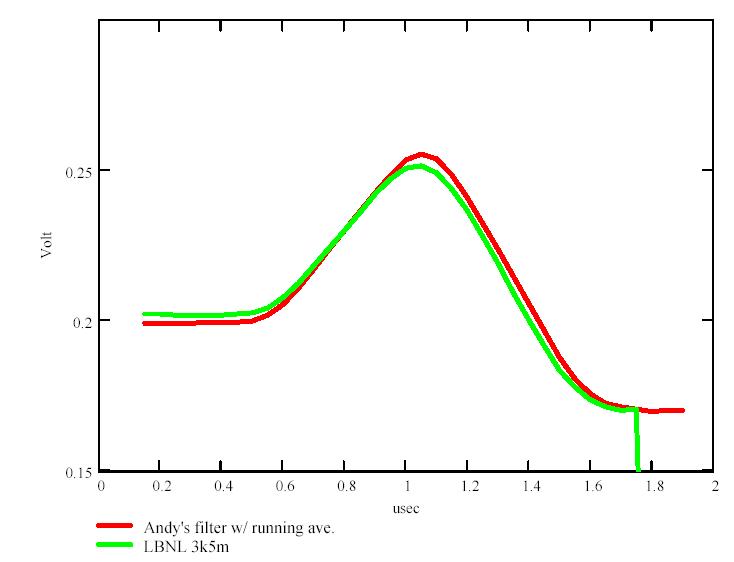
The response of Andy Laundrie's filter looks very much like the response of the 3.5km-long cable.
==================================================================================
Andy's Revised Filter
Andy Laudrie announced a revised component values on 2/19/2004 (read your email), saying that the previous design gave too fast a rise time in the response. As seen in the above plots, that doesn't seem to be the case. The actual response measured using the revised filter is shown below. The previous design seems to match the actual 3.5km cable response more closely than this revised version.
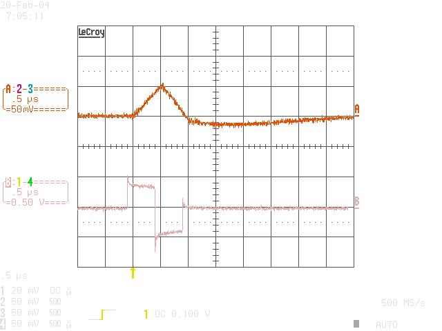 |
The input signal is distorted and has the amplitude smaller than what is programmed into the arbitrary waveform generator. The symptom is consistent with an impedance mismatch. The measurement was done in the identical setup as in the previous scope shot. |
The following is a comparison that after applying the running average to the scope data.
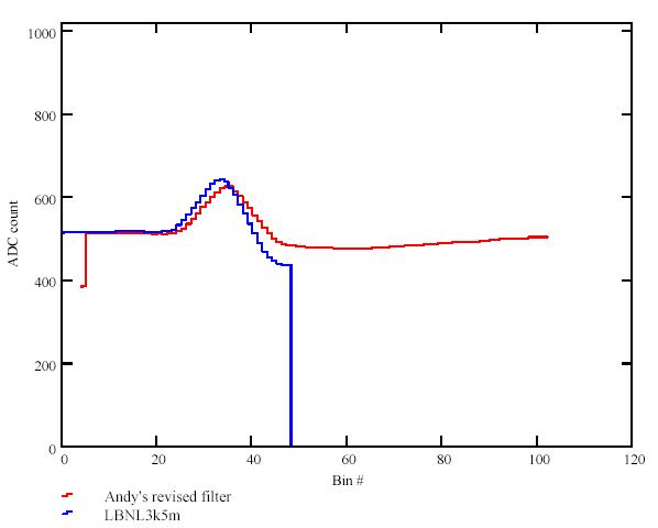
See more detail in the following files:
- MathCad calculation of the running average:revised_filter/running_ave2.mcd
- Data for MathCad document: revised_filter/revised_filt.txt, revised_filter/LBNL3k5m.txt
- Excel sheet: revised_filter/comparison3.xls
===================================================================================
By the way, the following is still an unresolved mystery:
Comparison: RAPcal with Long Cable vs RAPcal with Filter
(The curves have been manually shifted in x-direction to overlap with one another.)
The large discrepancy in amplitude is a mystery !? at this time (2/13/2004).
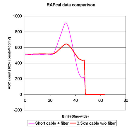
Excel datasheet: comparison2.xls