Interferometry
Related doc. Reco. workshop
Related code py_interferometers class
This is done by below command:
source ../setup.sh
python3 script_executor.py -k snr -s <station ID> -r <run number>                    # calculates SNR
python3 arr_time_table_maker.py <station ID>                                         # calculates arrivaltime table by ray tracing
python3 script_executor.py -k reco_ele_lite -s <station ID> -r <run number>          # performs vertex reconstruction based on AraCorrelator method
For sim:
source ../setup.sh
python3 sim_script_executor.py -k rms -s <station ID> -d <sim output path>            # both signal and noise. calculates rms
python3 rms_merge.py <station ID>                                                     # nosie only
python3 snr_maker.py <station ID> <rms results path>                                  # both signal and noise. calculates SNR by rms from noise event
python3 sim_script_executor.py -k reco_ele -s <station ID> -d <sim output path>       # both signal and noise. finds c_max of all elevation angle
User can find arrival time table from /data/ana/ARA/ARA02(or 3)/arr_time_table/arr_time_table_A2(or 3)_all.h5
Calculates the summed-cross correlation at a grid of pixels (theta, phi) for a source at fixed radius.
If signal is coming certain source, same type of antennas will have a similar WFs
By ray tracing algorithm, we can estimate arrival time differences of all air/ice positions
Cross-correlating WFs by removing arrival time differences, we can get correlation coefficient of all air/ice positions
Most highest coefficient score (Cmax) would be the reconstructed source position
5 radius (41, 170, 300, 450, 600 m), Direct / Reflect rays, D / R / D+R map, and default ice model were used for interferometry.
Detail Equations
Each cross-correlation ‘bin’ is normalized by product of sqrt of power.
Hilbert envelope is applied on each cross-correlation
Cross-correlation of all pairs are weighted by product of SNR.
Most highest coefficient score (Cmax) was chosen as reconstructed source position
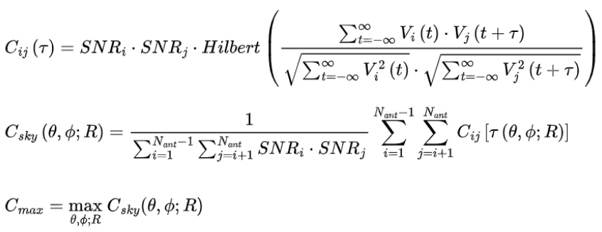
Fig. 89 interferometry equations
Calpulser example
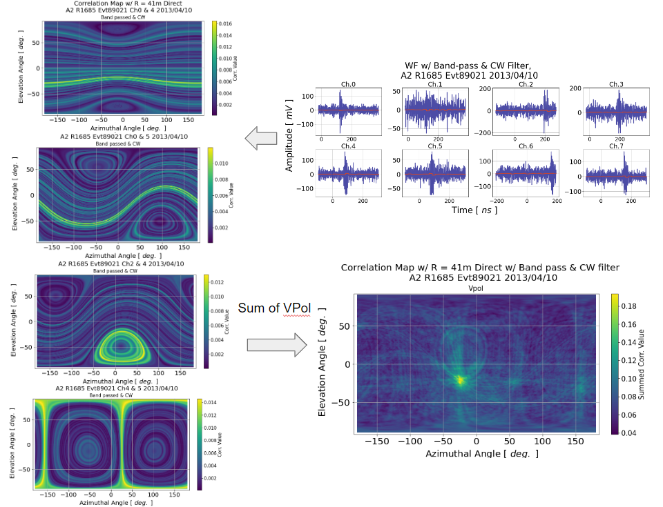
Fig. 90 calpulser example
Template Analysis
Related code ara_matched_filter class
User must generate the template by AraSim. Setup file for template: A2 and A3
This is done by below command:
source ../setup.sh
python3 arr_time_table_maker.py <station ID>                                         # calculates arrivaltime table by ray tracing
python3 sim_script_executor.py -k temp -s <station ID> -d <sim output path>           # both signal and noise. generates template that will be used for matched filter to data and sim
python3 sim_script_executor.py -k mf -s <station ID> -d <sim output path>             # both signal and noise
python3 script_executor.py -k mf -s <station ID> -r <run number>                     # perform matched filter
Searching for Neutrino signal by directly comparing with Neutrino template
Aiming to find low SNR signal
Simulated Neutrino templates
Preparing the expected Neutrino WFs that we can get from ARA
On/off-cone, shower, zenith gain pattern, and electronic response
Matched filtering technique
Cross-correlating data and template set while suppressing noise by noise model
Event-wise MF value (Mmax)
Summing up matched filter results (M(t)) after removing arrival time delay
Cons. of this analysis is, it is model dependent. Currently, I’m using the AraSim model. Single model dependency will be dealt with as an systematic uncertainty
Template Parameter
Four parameters for constructing template sets (total 24 WFs per channel)
Signal chain gain: 16
Zenith dependent antenna gain pattern: 4 (30, 50, 70, 90 deg)
On/Off-cone angle: 3 (0, 2, 4 deg)
Electromagnetic (EM) and hadronic (HAD) shower models: 2
Neutrino energy and the distance from the vertex to the detector, can be simplified using a scale factor.
Shape differences of Askaryan cut-off per energy/off-cone are not considered
Receiving angle, -60, -40, -20, and 0, and On/Off-cone angle, 0, 2, and 4, are used for template set
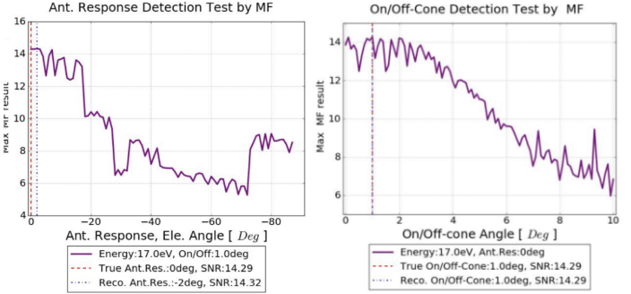
Fig. 91 template parameter test results
Detail Equations
Cross-correlation between data and template in f-domain with Hilbert envelope
Suppress noise (weighting) in the f-domain by power spectral density (PSD) (averaged software triggered data)
Averaged software triggered data (Rayl. x sqrt(pi / 2))
Normalizes template and PSD amplitude (alpha_n)
Sums up correlation results (Msum) after removing arrival time delay (tau_n) from AraSim ray tracing
Most highest coefficient score (Mmax) was chosen for the event-wise result
Cons. of template analysis is, it is model dependent. Currently, I’m using the AraSim E-field model
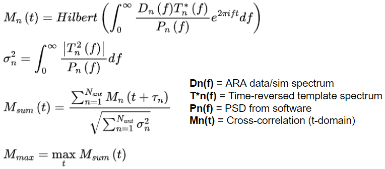
Fig. 92 matched filter equations
Event-wise Matched Filter
192 (8 chs * 24 templates) MF results are reduced to ‘single’ value (But total 2 by V/HPols)
Off-cone dim. is reduced in individual channel level
Channel dim. is reduced by summing up after removing arrival time delay
total 84 summed results by 2 shower, 7 zenith, and 6 azimuth
Summing is done by ~80 ns of rolling maximum
Among the 84 summed results, I choose 1 result that has maximum Mmax value
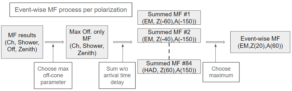
Fig. 93 event-wise matched filter process
Simulation example
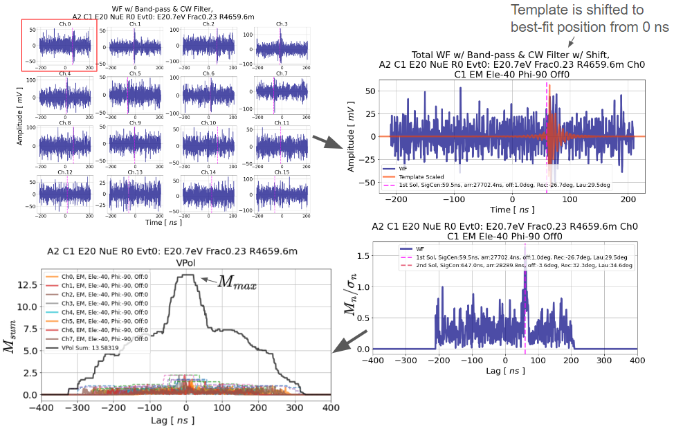
Fig. 94 simulation results
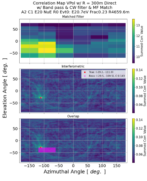
Fig. 95 simulation results with vertex reconstruction compare to interferometry