Preparation

In order to perform signal background saparation, User must merge all the results into single files

Results of 100 million events (per station) that needed for signal background saparation cut: run number, event number, trigger type, unix time, live time, quality cut (33 cuts), interferometry (2 pols), and matched filter (2 pols)

Numpy array that has 100 million elements in float format is equal to 1 GB. So, It is easily handle all of them at once

This is done by below commands

For the data side:

source ../setup.sh
python3 script_executor.py -k sub_info_burn -s <station ID> -r <run number>          # collect sencondary information in the burn sample
python3 info_summary.py <station ID>                                                 # collect run and event number, trigger type, and unxi time for all events
python3 dat_summary_live.py <station ID> <entry> <entry width>                       # calculates live time based on 1st data cleaning
python3 dat_summary_live_sum.py <station ID>                                         # merges the results
python3 dat_summary_qual.py <station ID> <entry> <entry width>                       # collect the data cleaning results of all events
python3 dat_summary_qual_sum.py <station ID>                                         # merges the results
python3 dat_summary.py <station ID> <entry> <entry width>                            # collect the vertex reconstruction and matched filter results of all events
python3 dat_summary_sum.py <station ID>                                              # merges the results

For the simulation side:

source ../setup.sh
python3 sim_summary_qual.py <station ID> <signal or noise>                            # both signal and noise. collect the data cleaning results of all events
python3 sim_summary.py <station ID> <signal or noise>                                 # both signal and noise. collect the vertex reconstruction and matched filter results of all events

Results of all 3 data cleanings in 2 parameter space

This is done by Check_Sim_v30_mf_corr_2d_map_final_surface_cut_total

Results of evolution of cuts in the space of two event selection methods

Interferometric in x-axis and matched filter in y-axis
All configurations are merged in one dataset

Remaining data is most likely consist to thermal noise

Signal/background cut is defined in this space

../../_images/sb_hist_0.png — Fig. 96 Evolution of data cuts. A2 VPol

../../_images/sb_hist_1.png — Fig. 97 Evolution of data cuts. A2 HPol

../../_images/sb_hist_2.png — Fig. 98 Evolution of data cuts. A3 VPol

../../_images/sb_hist_3.png — Fig. 99 Evolution of data cuts. A3 HPol

Diagonal Cut in 2 parameter space

Making/Optimizing the diagonal cut in Cmax vs Mmax space for signal/background separation

Makes diagonal cut by optimizing y = a * x + b. a: slope and b: intercept

Decided to make a signal/background cut by adding up all configurations (global cut)

More conservative approach
Testing various slope and intercept parameters: 2d grid search

Cut will be optimized by more broad distribution

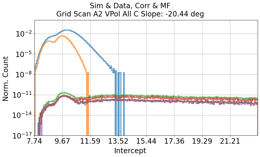
../../_images/sb_hist1_0.png — Fig. 100 Projected data and simulation based on slope and intercept parameter

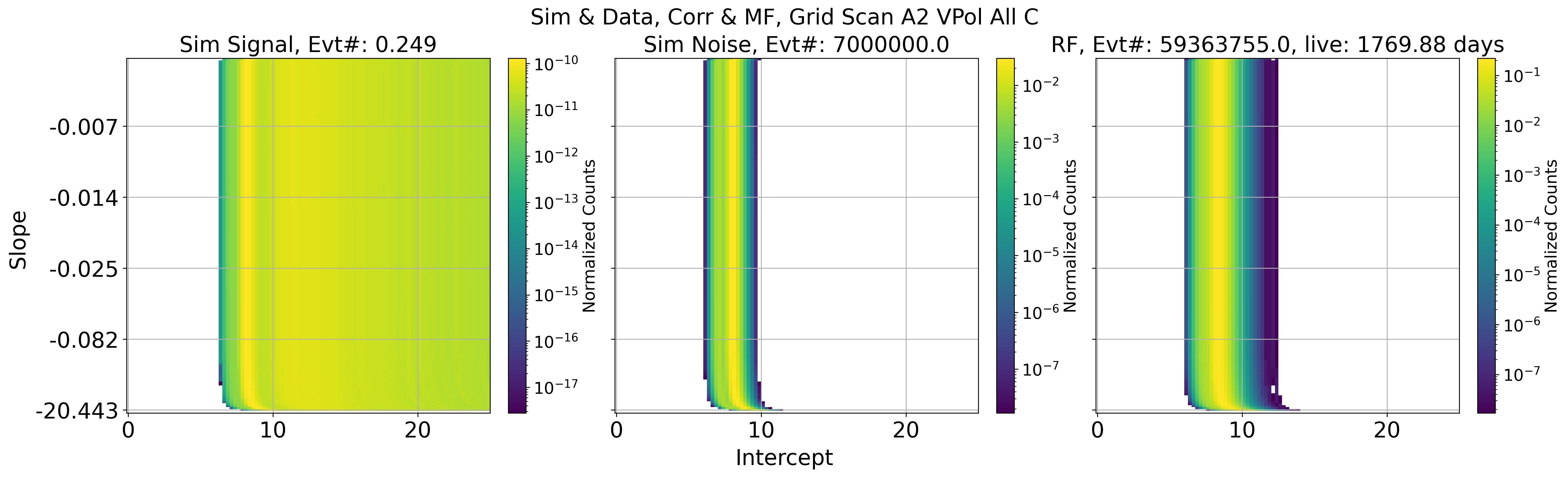
../../_images/sb_hist1_1.png — Fig. 101 A2 VPol. Projected data and simulation based on all slope and intercept parameter

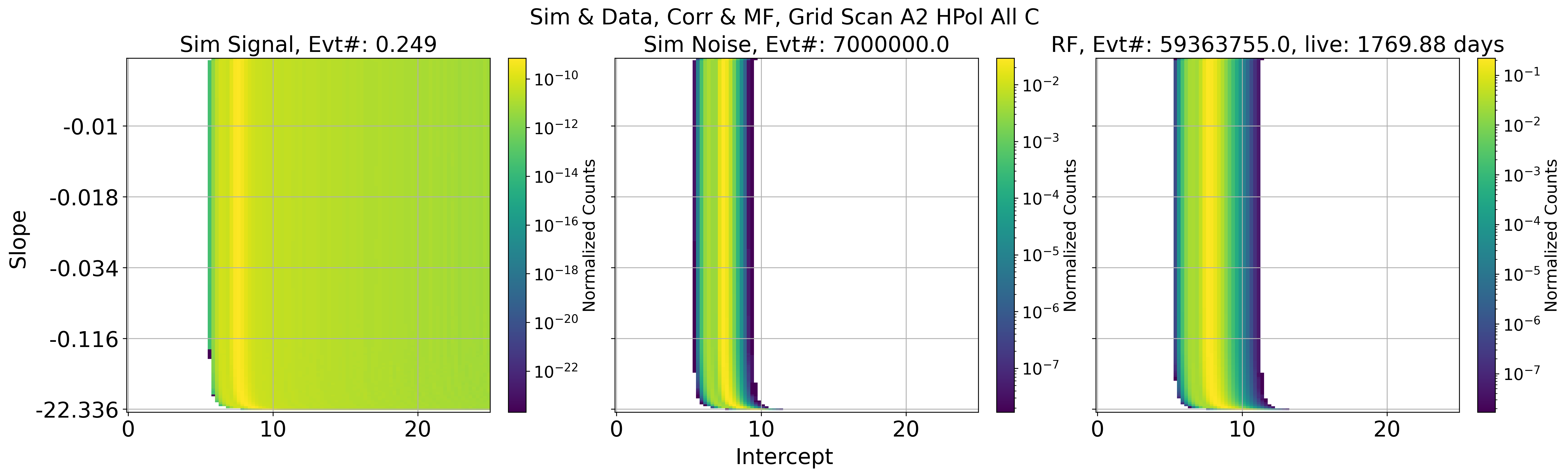
../../_images/sb_hist1_2.png — Fig. 102 A2 HPol. Projected data and simulation based on all slope and intercept parameter

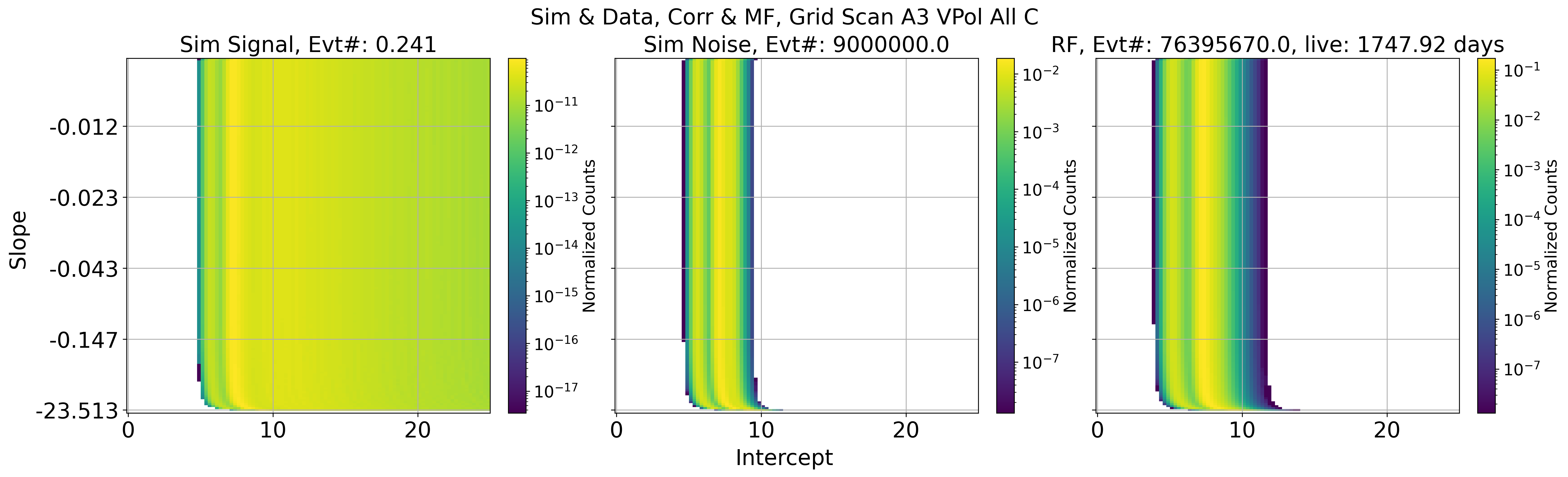
../../_images/sb_hist1_3.png — Fig. 103 A3 VPol. Projected data and simulation based on all slope and intercept parameter

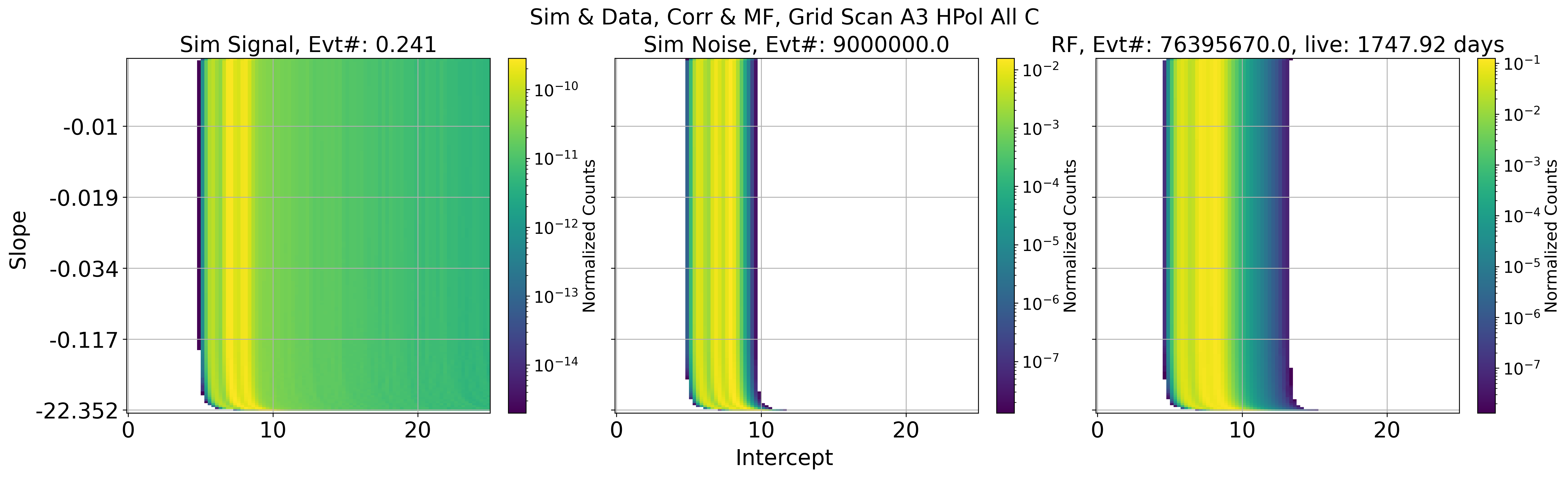
../../_images/sb_hist1_4.png — Fig. 104 A3 HPol. Projected data and simulation based on all slope and intercept parameter

Goodness of fit

This is done by back_est_gof_ell.py and back_est_gof_ell_sum.py

In each slope, exponential fit is performed.

y = p0 * exp(-p1 * (x - xmin)). xmin: fit starting point

Calculates -2log(L) values of pseudo-experiment (10k) created by fit

Check where -2log(L) of actual data can be landed in the pseudo-distribution
If p-value is bigger than 0.05, it is acceptable fit that can describe the data

Procedure is,

Integral the fit region to get expected # of background
Apply poisson dist. by using ‘expected # of background’ as 𝝺
(Randomly) generate K amount of data by following fit line -> pseudo-experiment
Computing log-likelihood between Pseudo data and fit
Do this many times

In order to confirm which data region is proper to use for fitting, Above procedure also repeated by 20 different data region (dividing range between max peak to last data point into 20)

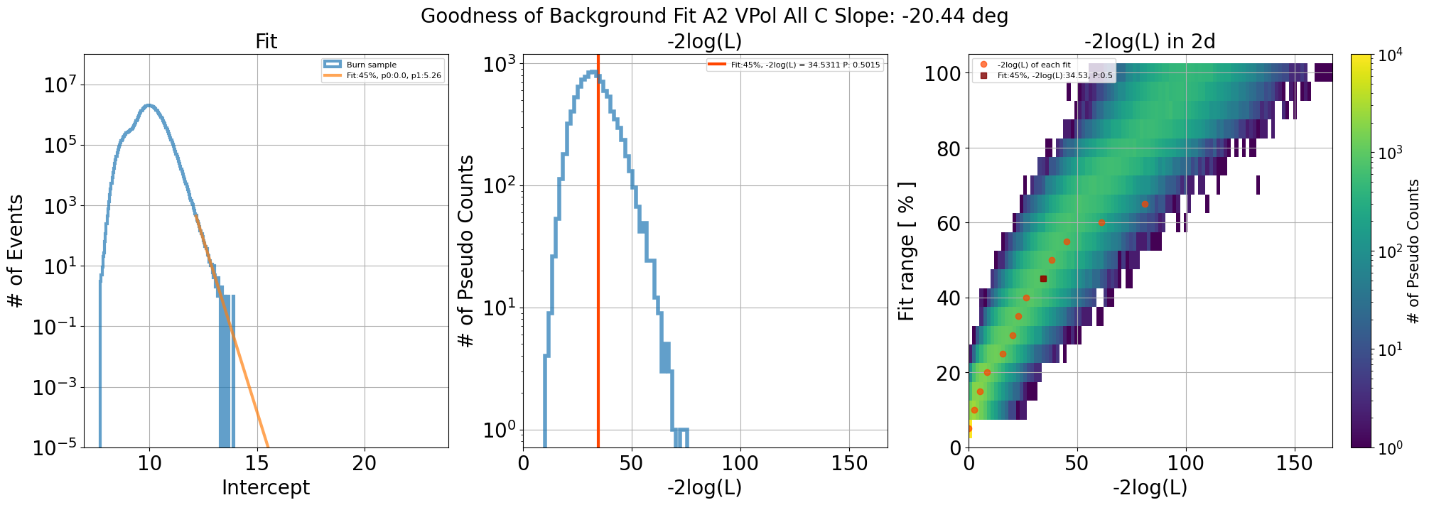
../../_images/sb_hist2_0.png — Fig. 105 Left: data distribution and fit including parameters. Middle: Result of pseudo-experiment including p value. Right: Result of pseudo-experiment into 2d histogram. p value that close to 0.5 is selected for estimating background

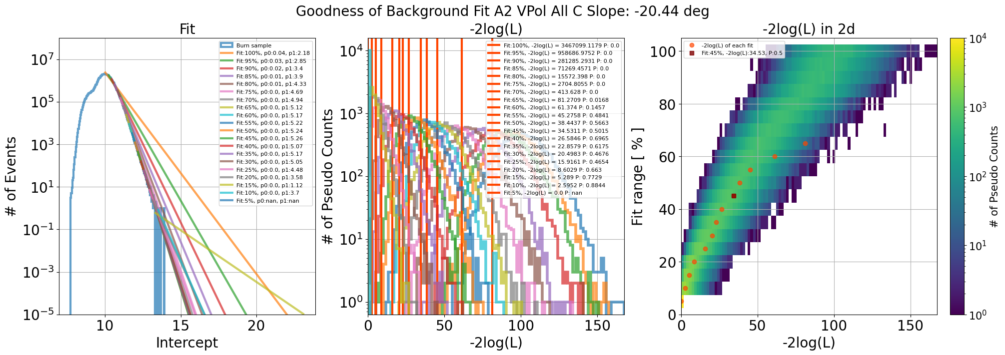
../../_images/sb_hist2_1.png — Fig. 106 Left: fit results with 20 different data range. Middle: Result of pseudo-experiment. Right: Result of pseudo-experiment into 2d histogram. p value that close to 0.5 is selected for estimating background

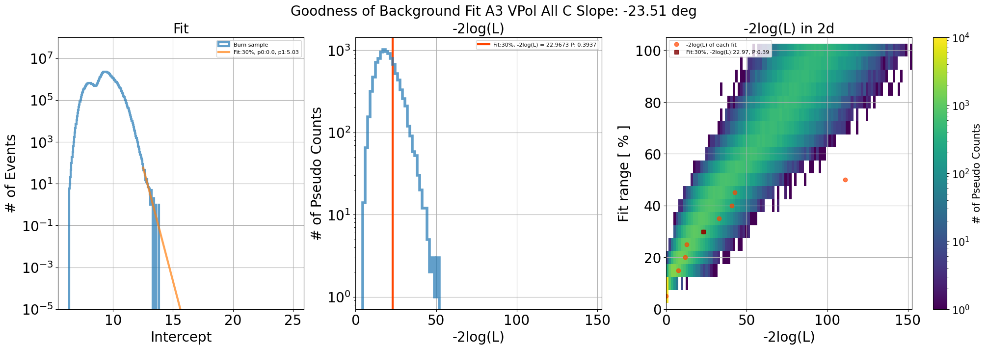
../../_images/sb_hist2_2.png — Fig. 107 A3 VPol

../../_images/sb_hist2_3.png — Fig. 108 A3 VPol with all data range

Background Estimation

This is done by Check_Sim_v32.2_back_est_pseudo_total_w_edge_ellipse

Performs pseudo-experiment to estimate background estimation

Creates 100k of different fit line by using gaussian distribution

p0 and p1 are means and uncertainty of each parameter are sigma
sigam is calculated by uncertainty and correlation coefficient of parameter

Calculates 100k of background number for each intercept cut values

Each intercept cut values, choose median as an background estimation and 1 sigma from median as an error

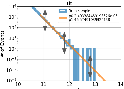
../../_images/sb_hist3_0.png — Fig. 109 Illustration of fluctuation of fit

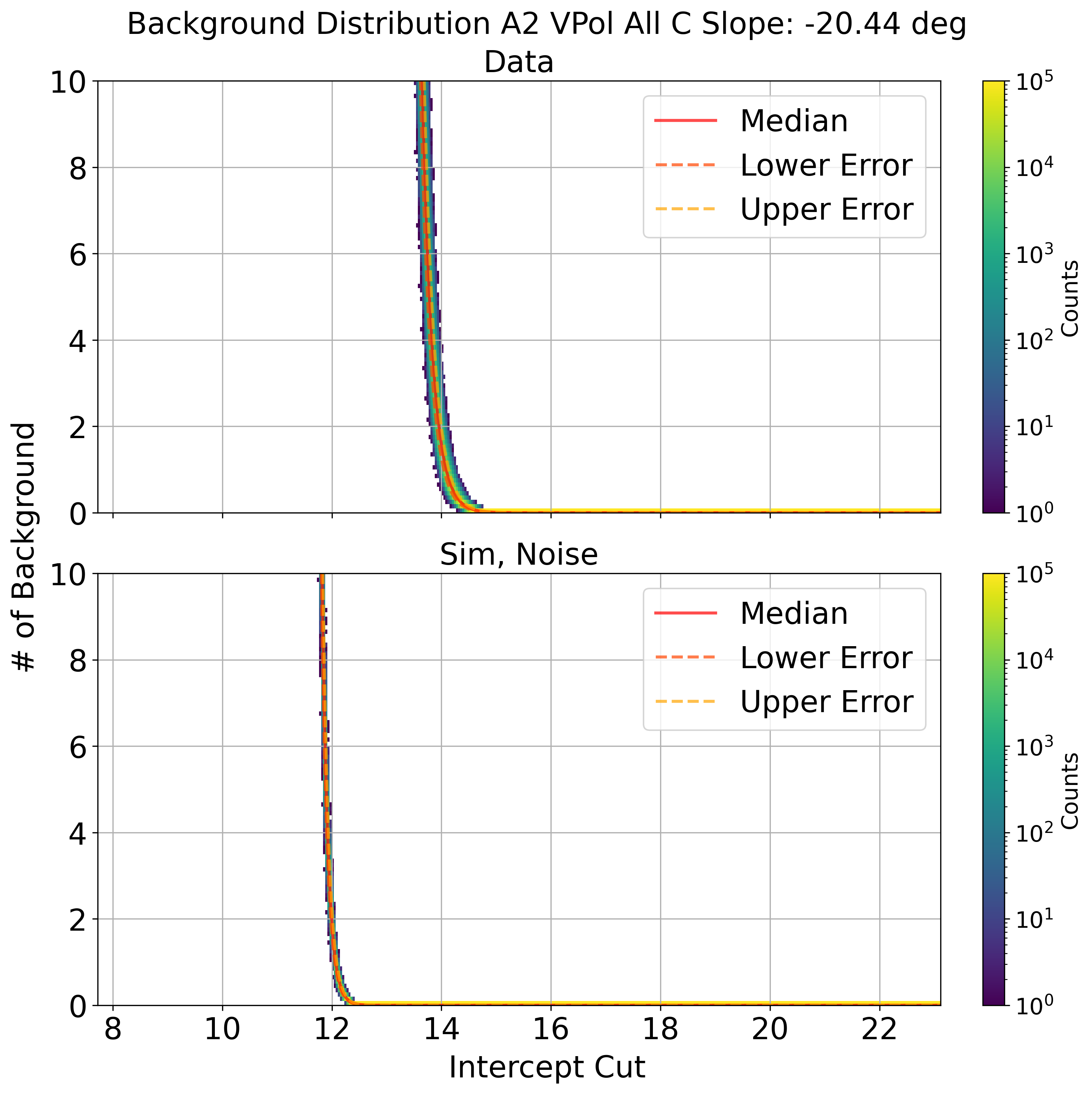
../../_images/sb_hist3_1.png — Fig. 110 background estimation data and noise sim by pseudo-experiment

Upper Limit

This is done by upper_limit_summary_total.py

Use results of back.est. to run another 10k pseudo exp. by poisson distribution

Considering zero signal detection

Use K from poisson dist. to run Feldman Cousin method

Mean value of upper limit distribution by 10k pseudo exp. was used for final value

Cut value that has maximum ratio of S / Sup would be optimal upper limit position

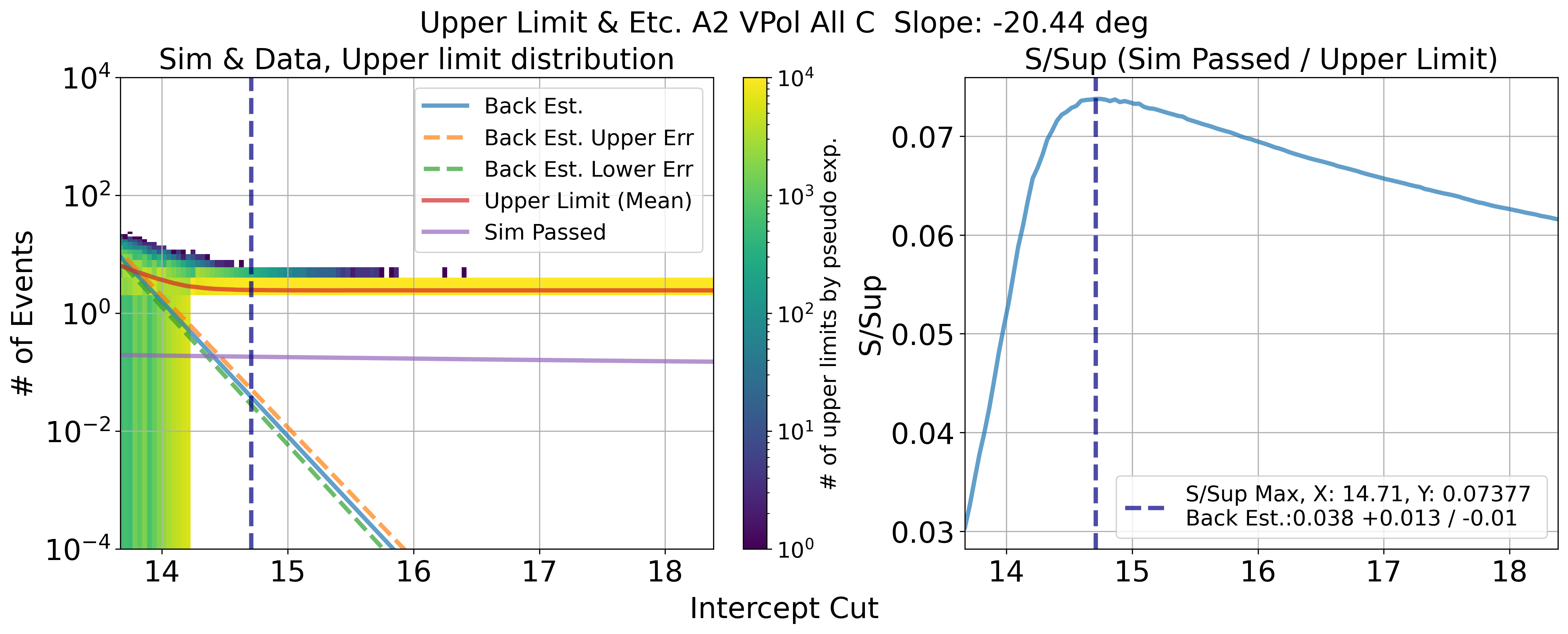
../../_images/sb_hist4_1.png — Fig. 111 A2 VPol. Results of upper limit and s / sup. maximum s / sup ratio is final cut value

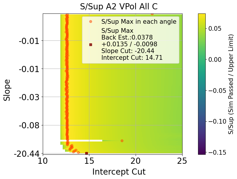
../../_images/sb_hist4_0.png — Fig. 112 A2 VPol. s / sup ratio in all slope

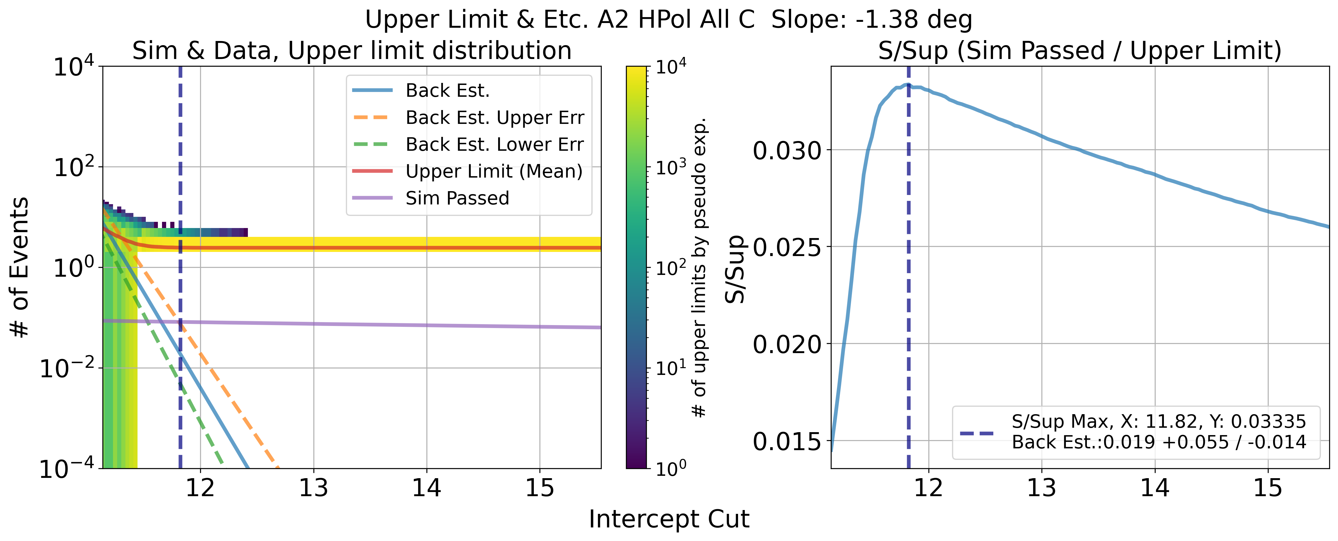
../../_images/sb_hist4_3.png — Fig. 113 A2 HPol. Results of upper limit and s / sup. maximum s / sup ratio is final cut value

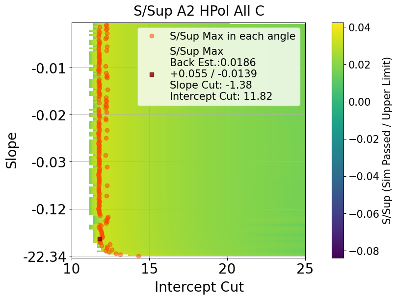
../../_images/sb_hist4_2.png — Fig. 114 A2 HPol. s / sup ratio in all slope

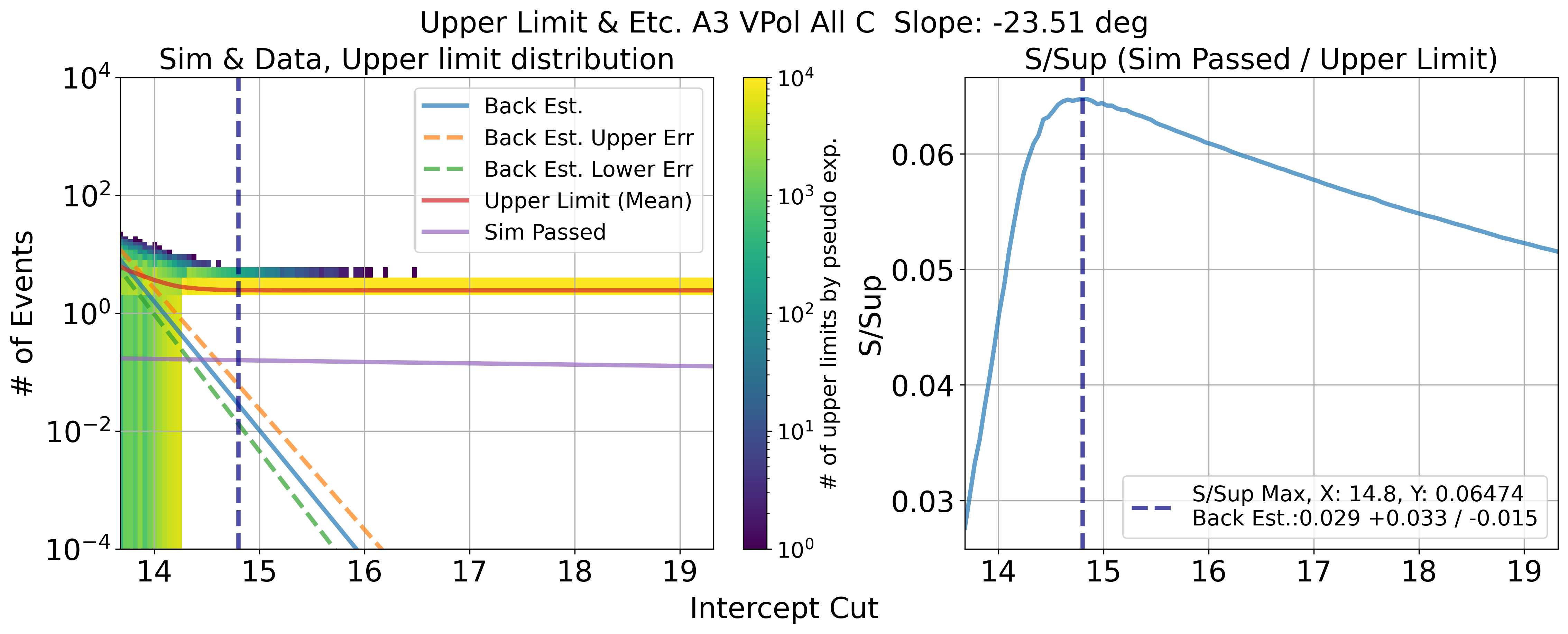
../../_images/sb_hist4_5.png — Fig. 115 A3 VPol. Results of upper limit and s / sup. maximum s / sup ratio is final cut value

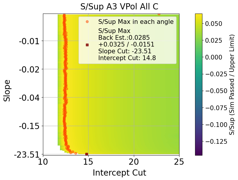
../../_images/sb_hist4_4.png — Fig. 116 A3 VPol. s / sup ratio in all slope

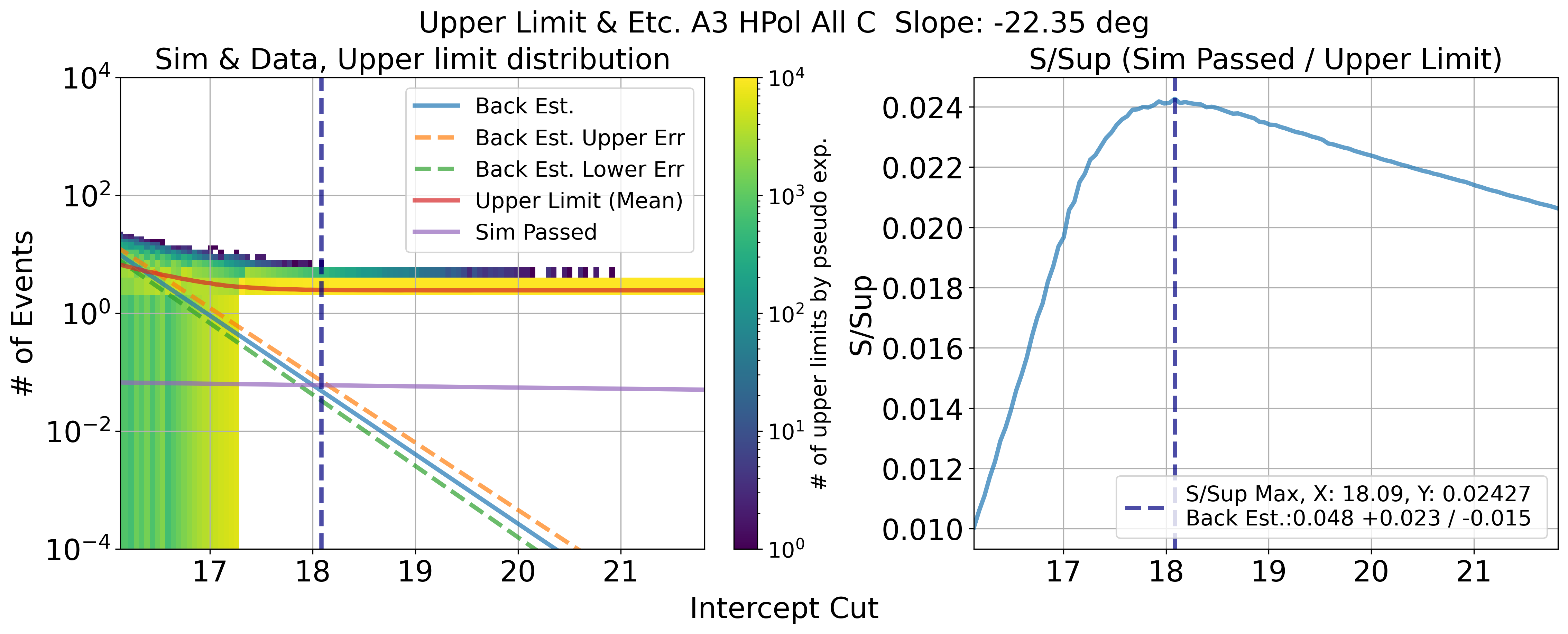
../../_images/sb_hist4_7.png — Fig. 117 A3 HPol. Results of upper limit and s / sup. maximum s / sup ratio is final cut value

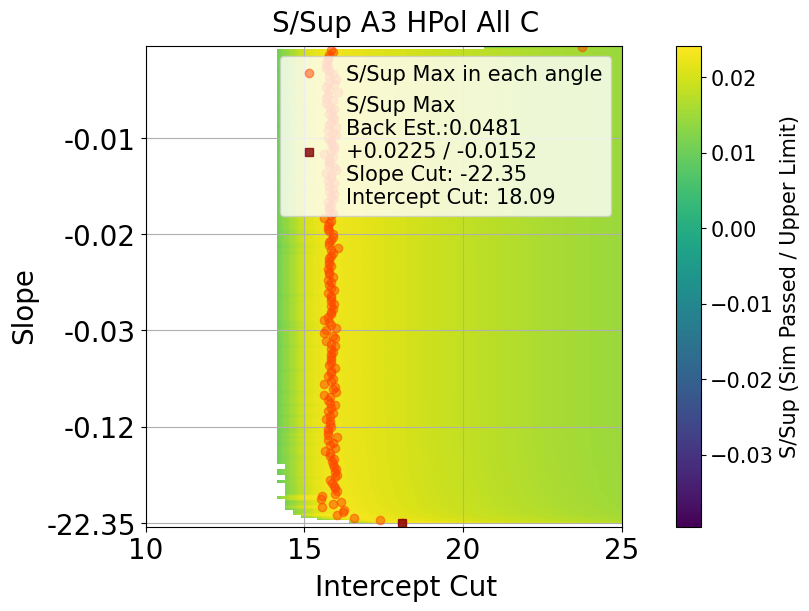
../../_images/sb_hist4_6.png — Fig. 118 A3 HPol. s / sup ratio in all slope

Results of signal / background cut in 2 parameter space

This is done by Check_Sim_v34.3_mf_corr_ver_2d_map_w_cut_combine_w_noise_total_w_edge_ellipse

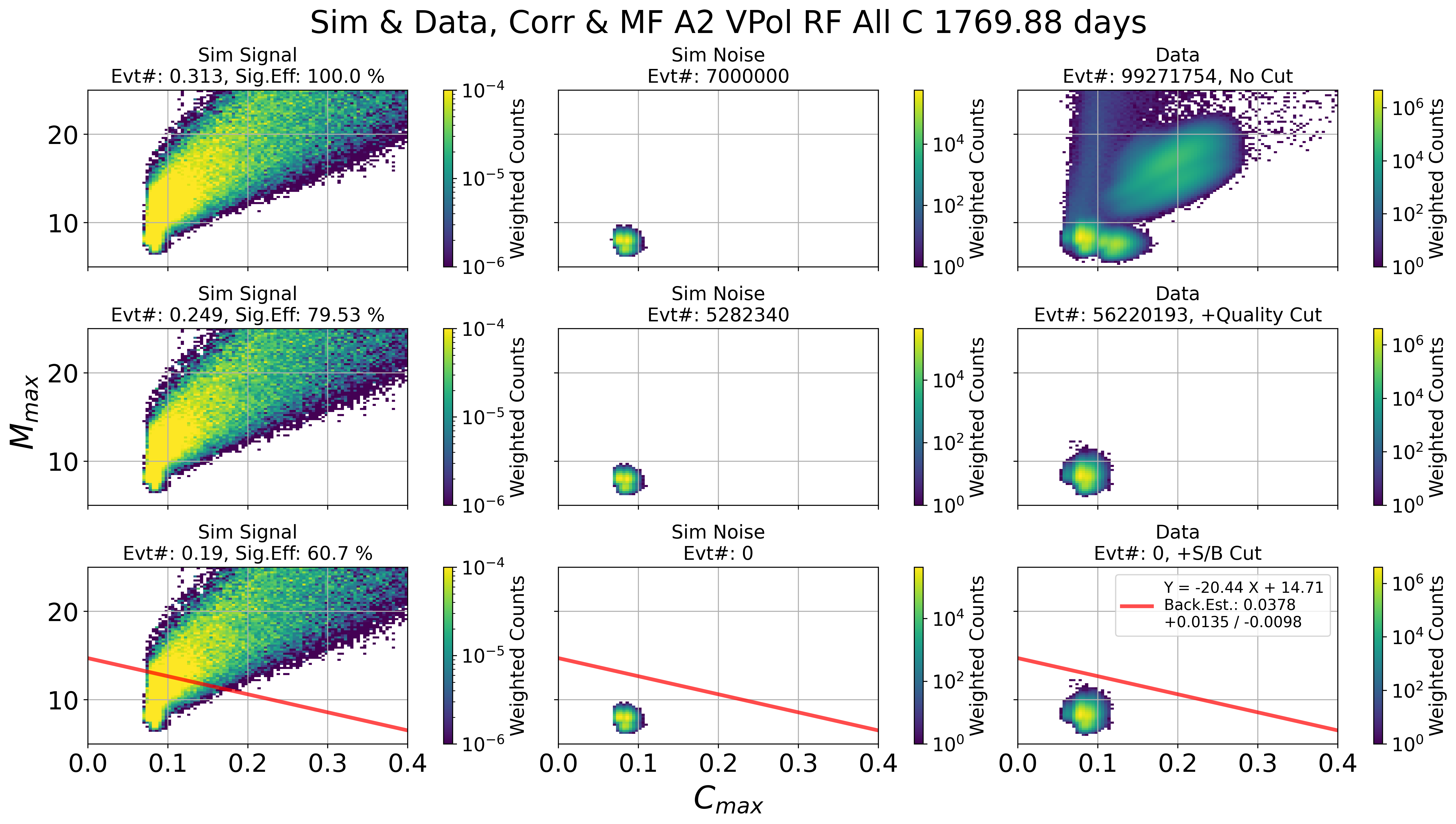
../../_images/sb_hist4_8.png — Fig. 119 A2 VPol. Left: sim signal. Middle: sim noise. Right: data

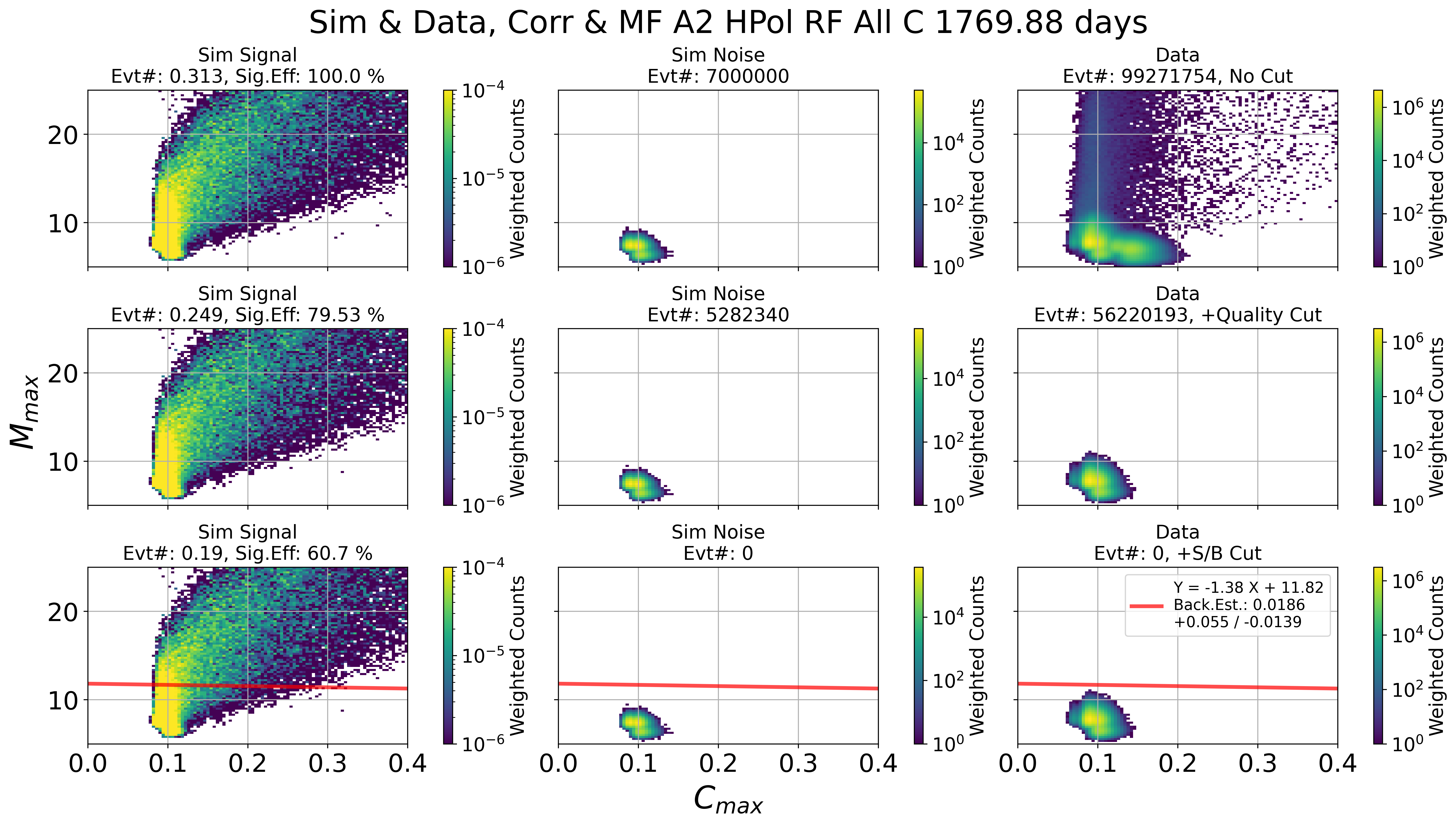
../../_images/sb_hist4_9.png — Fig. 120 A2 HPol. Left: sim signal. Middle: sim noise. Right: data

../../_images/sb_hist4_10.png — Fig. 121 A3 VPol. Left: sim signal. Middle: sim noise. Right: data

../../_images/sb_hist4_11.png — Fig. 122 A3 HPol. Left: sim signal. Middle: sim noise. Right: data

Passed simulation event

This is done by Check_Sim_v34.3.2_mf_corr_ver_pos_total

../../_images/sb_hist555_0.png — Fig. 123 A2. passed simulated events by 3 different steps

../../_images/sb_hist555_1.png — Fig. 124 A3. passed simulated events by 3 different steps

Left col.: Radius vs Depth map. Station is located the zero position

Middle col.: Energy vs Radius map

Right col.: Vertex theta/phi position differences between reco (interferometric) and true

Most of event we will see is corresponding to depth above -2000 m and energy below 10^11 eV

Tail to up on elevation angle differences are coming from mis-reconstruction of surface reflected event

Sanity check of AraCorrelator and AraVertex

Below plots are sanity check of our vertex reconstruction methods. 2d map is the reconstructed elevation angle against the true elevation angles. 1d map is differences bwteern reconstructed and true.

I didnt exactly saparate the event based on their polarization. So, for example, half circle shape of distribution in AraCorr V is not caused by mis-reconstruction. It has strong HPol signal and weak VPol signal.

Except polarization issue, Typical three branch distribution in each plot (streched from center to bottom left, top right and top left) is similar to testbed publication. Top left branch is caused by general mis-reconstruction of surface reflected event.

In A3, the mis-reconstruction, specially in AraVer V, in config 6 to 9 is caused by the channel that experiencing amplifier failure

If below plots are too hard to see, you can find high resolution one in here: A2 and A3

../../_images/sb_hist5_2.png — Fig. 125 A2. True vs Reco elevation angle. 1st: VPol results from AraCorrelator, 2nd: HPol results from AraCorrelator, 3rd: VPol results from AraVertex, 4th: HPol results from AraVertex, 5th: V+HPol results from AraVertex

../../_images/sb_hist5_3.png — Fig. 126 A2. True - Reco elevation angle. 1st: VPol results from AraCorrelator, 2nd: HPol results from AraCorrelator, 3rd: VPol results from AraVertex, 4th: HPol results from AraVertex, 5th: V+HPol results from AraVertex

../../_images/sb_hist5_4.png — Fig. 127 A3. True vs Reco elevation angle.

../../_images/sb_hist5_5.png — Fig. 128 A3. True - Reco elevation angle.

Below plots are comparison of reconstructed vertex positions bewtween AraCorrelator and AraVertex

Both methods have different search condition

AraCorrelator search through all theta and phi with 1 degree resolution. But I limited radius to 41, 170, 300, 450,and 600 m
AraVertex search conditions are 1) ice model parameter is changed to match with AraSim default model iceProp(1.78,-0.43, 0.0132). 2) radius search range is 170 to 5000 m. 170 m is set to prevent mis_reconstruction. If I set minimum range to original value, often surface events are reconstructed to close to antenna and have a elevation angle clode to 0 degree. 3) RPR threshold is set to 4 and minimum number of antenna that requried to perform Aravertex is set to 3. It is for catching surface event that has low SNR.

Due to radius conditions of both methods, depth results, which is driven from theta and radius results, are has discripancy. but most of discripancy is casued by very low SNR event.

../../_images/sb_hist5_6.png — Fig. 129 A2. 1st: VPol results of theta comaprison. 2nd: HPol results of theta comaprison. 3rd: VPol results of depth comaprison. 4th: HPol results of depth comaprison.

../../_images/sb_hist5_7.png — Fig. 130 A2. 1st: VPol results of theta differences. 2nd: HPol results of theta differences. 3rd: VPol results of depth differences. 4th: HPol results of depth differences.

../../_images/sb_hist5_8.png — Fig. 131 A3

../../_images/sb_hist5_9.png — Fig. 132 A3

Summary of backgound estimation and signal efficiency

A2

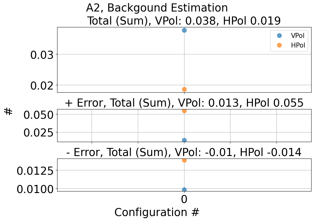
../../_images/sb_hist6_0.png — Fig. 133 A2 backgound estimation

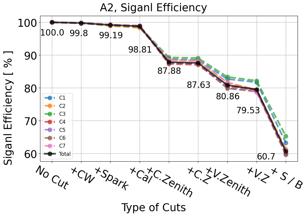
../../_images/sb_hist6_1.png — Fig. 134 A2 signal efficiency

A3

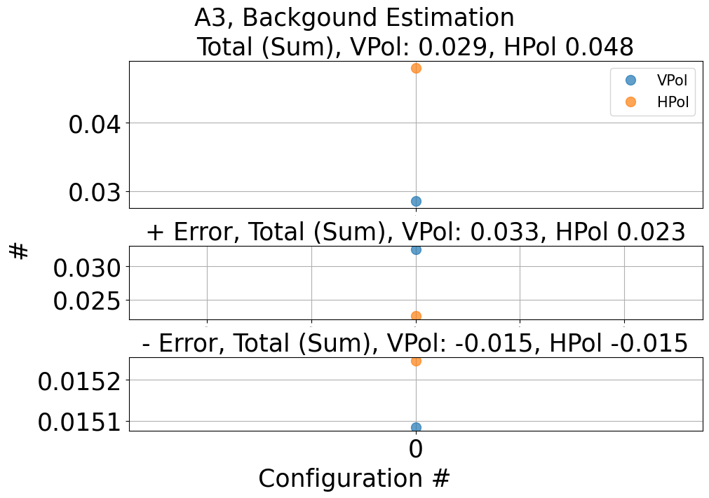
../../_images/sb_hist6_2.png — Fig. 135 A3 backgound estimation

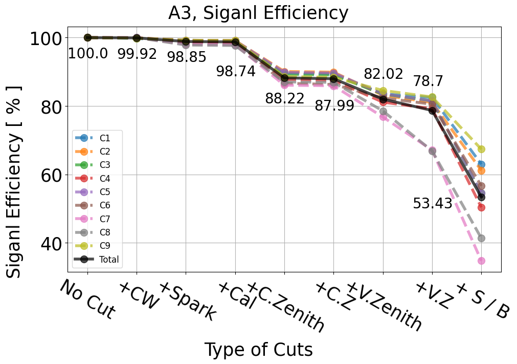
../../_images/sb_hist6_3.png — Fig. 136 A3 signal efficiency