Effective Area Estimation

Concept

Unfolding the muon’s true propagation length and surface energy from the network’s estimations yields results that are given as distributions of events per time unit, e.g. in units of \(\frac{1}{s}\). This is referred to as an event rate and merely describes the number of measured events in a certain time. Since detectors are not perfectly sensitive and also not every muon from the surface actually reaches the detector, it is important to convert these simple event rates to fluxes with units of \(\mathrm{m}^{-2} \mathrm{s}^{-1} \mathrm{sr}^{-1} \mathrm{m.w.e.}^{-1}\) by means of an effective area. The effective area takes into account the different detector/analysis specific detection efficiencies, thus making the resulting distributions comparable between different detectors and analyses. The event rates are bin-wise converted to fluxes via

\[\begin{equation} \Phi_{i} = \frac{N_{i}}{T \cdot \Delta L_{i} \cdot \Omega_{i} \cdot A_{\mathrm{eff},i}} \; , \end{equation}\]

where \(N\) denotes the number of events, \(T\) the livetime, \(\Delta L\) the binwidth, \(\Omega\) the solid angle and \(A_{\mathrm{eff}}\) the effective detection area for each bin \(i\). The solid angle is calculated according to

\[\begin{equation} \Omega_{i} = 2 \pi \cdot \left(\cos{\Theta_{\mathrm{min}, i}} - \cos{\Theta_{\mathrm{max}, i}}\right) \; , \end{equation}\]

with \(\Theta_{\mathrm{min},i}\) and \(\Theta_{\mathrm{max},i}\) as the minimum and maximum zenith angle of the propagation length bin. The effective area takes the detection efficiency into account and is calculated on simulation data by rescaling the detector area with the fraction of selected to generated events. The general idea follows the approach

\[\begin{equation} A_{\mathrm{eff}} = A_{\mathrm{sim}} \frac{N_{\mathrm{sel}}}{N_{\mathrm{gen}}} \; , \end{equation}\]

where \(A_{\mathrm{sim}}\) is the detector area perpendicular to the corresponding muon trajectory (also shown in Fig. 38), \(N_{\mathrm{sel}}\) is the number of selected events and \(N_{\mathrm{gen}}\) is the number of generated muons on the plane. Dividing the event rate by the effective area enables to trace the number of detected events back to the number of all arriving muons per unit area.

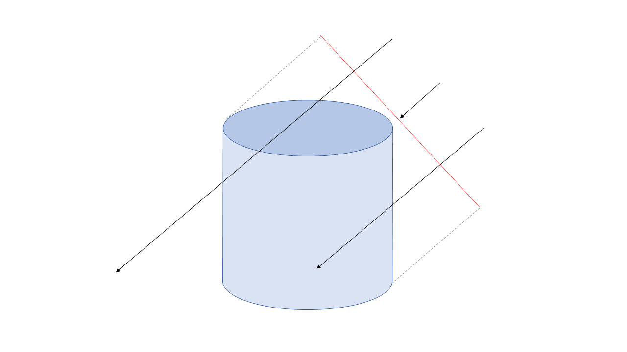
Fig. 38 : Schematic representation of the detector area perpendicular to the muon trajectory (red line). The number of generated muons \(N_{\mathrm{gen}}\) amounts to the number of all particles with a trajectory through that plane, regardless of whether they reach the detector or not (black arrows). The projected area depends on the direction of the particles.

The stopping muon depth intensity as well as the surface energy spectrum agree in the sense that both result from muons with very different properties in terms of energy and track length through the ice. Hence, if one thinks of a number of muons being generated on a 2D plane (defined at a certain depth in the ice), the fluxes span from muons stopping far in front of the plane up to muons stopping far behind the plane, as shown in Fig. 38. The detector area \(A_\mathrm{sim}\) is always defined perpendicular to the corresponding muon tracks, as it becomes independent of how far the muons propagate this way.

In our most general approach of calculating \(A_{\mathrm{eff}}\), we count every one of the muons \(N_{\mathrm{gen}}\) that were simulated at the surface. Here, the effective area is not defined in the classical sense of only accounting for the detection probability, but also serves as a correction factor to the number of muons that IceCube simply can not measure, because they do not reach the instrumented volume. However, if these muons are generated on the defined 2D plane and belong to a certain propagation length bin, they need to be included to retrieve the expected stopping muon intensity. These calculations have to be made on MC data since only simulations provide the necessary information about the existence of muons at the surface.

In order to restrict the number of generated muons \(N_{\mathrm{gen}}\) to particles that are more closely related to the stopping muon events that IceCube actually measures (muons stopping inside the instrumented volume), this general calculation is further adjusted. Further details on both approaches are given below. However, it should be noted here that they yield almost identical results.

Application to the Stopping Muon Sample

The effective area is calculated for each propagation length bin individually. Since the detector area perpendicular to the muon track \(A_{\mathrm{sim}}\) also depends on the zenith angle, \(A_{\mathrm{eff}}\) is calculated in two dimensions and then marginalized over \(\Theta\).

The selected events \(N_{\mathrm{sel}}\) and initially generated muons \(N_{\mathrm{gen}}\) are filled into 2-dimensional histograms of propagation length \(L\) and zenith angle \(\Theta\). This results in two 2D maps, that are used to calculate the fraction in the above equation in a multidimensional fashion. This yields

\[\begin{equation} A_{\mathrm{eff}}(L, \Theta) = A_{\mathrm{sim}}(\Theta) \cdot \frac{N_{\mathrm{sel}}(L,\Theta)}{N_{\mathrm{gen}}(L,\Theta)} \; . \end{equation}\]

Note that \(N_{\mathrm{sel}}\) counts selected events and \(N_{\mathrm{gen}}\) counts individual muons. This accounts for the muon multiplicity, as an event may contain multiple muons. Since IceCube’s file structure is based on the primary cosmic ray particle, each event corresponds to a single primary, but the primary may produce multiple muons. In order to calculate the depth intensity of atmospheric muons it is necessary to count each muon individually. The properties are known from the I3MCTree. Each individual muon is assigned with the weight of the corresponding event.

To obtain a weighted average per propagation length bin, the resulting effective area is marginalized over \(\Theta\), using the pdf of the generated events

\[\begin{equation} p(L, \Theta) = \frac{N_{\mathrm{gen}}(L, \Theta)}{\sum_\limits{\mathrm{bin}(L)}N_{\mathrm{gen}}(L, \Theta)} \; . \end{equation}\]

Each bin entry is divided by the sum of events in the corresponding length bin, such that

\[\begin{equation} \int p(L_{i}, \Theta) \; \mathrm{d}\Theta = 1 \; . \end{equation}\]

The effective area then reads

\[\begin{equation} A_{\mathrm{eff}}(L) = \iint p(L, \Theta) \cdot A_{\mathrm{eff}}(L, \Theta) \; \mathrm{d}\Theta \; . \end{equation}\]

The result is used to perform the conversion from above.

Adjustment of the General Approach

As mentioned above, it is desired to take the number of generated muons \(N_{\mathrm{gen}}\) to be more closely related to the particles that IceCube can actually detect. Thus, the effective area approaches its classical meaning of a pure sensitivity (detection efficiency) correction. Ideally, the ‘generated’ events should amount to only the muons that stop inside the instrumented volume. The effective area for different length bins would then be calculated by taking events from different zenith bands, since inclined events should correspond to increasingly large propagation lengths. This is not entirely feasible due to geometrical reasons. If muons are simulated on the 2D detector area and belong to a certain \(L\) bin, the volume of this bin will always span certain overlap regions around the detector (see Fig. 39). As a result, \(N_\mathrm{gen}\) still does not only count muons that stop inside the instrumented volume. However, the corresponding muons stop much closer to the detector in this approach and makes it a useful consistency check.

The main difference to the general approach is that now only the muons in the corresponding \(z\) range (vertical stopping depth in detector coordinates) of the detector are included in \(N_{\mathrm{gen}}\):

\[\begin{equation} -600 \, \mathrm{m} \; < z \; < 600 \, \mathrm{m} \; . \end{equation}\]

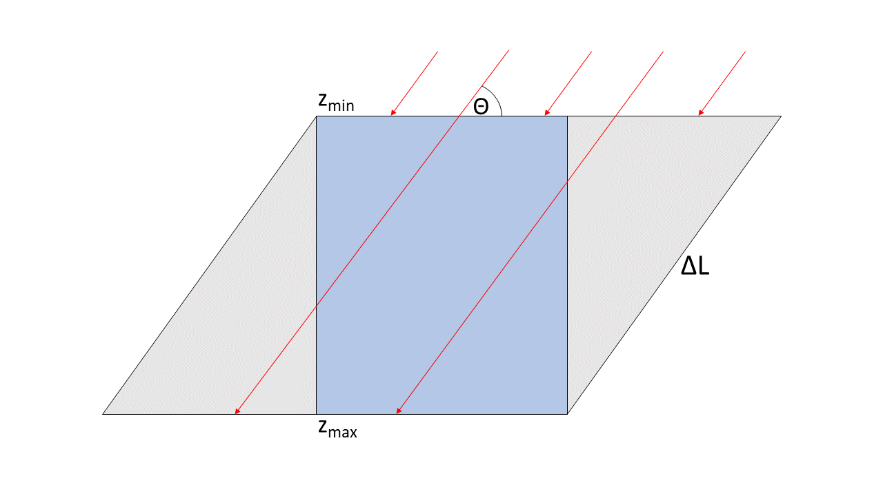
Fig. 39 : Schematic representation of a propagation length bin for a fixed muon direction. The instrumented detector volume is shown in blue (side view). Grey areas denote the volume that is covered by the length bin, but not by IceCube’s in-ice array. The geometry is defined by the the detector area perpendicular to the muon track and the limited \(z\) range. If the \(L\)-bin width is chosen to be smaller, the volume is compressed in the \(z\)-direction.

The overlap regions pose as a volume where the detector sensitivity equals zero, just as it is the case in the general approach. However, this overlap regions are reduced to a minimum region around the detector for the corresponding simulation area \(A_{\mathrm{sim}}\). The marginalization over \(\Theta\) works exactly the same way. The only difference lies in the pdf of the generated muons.

As shown in the Results section, the resulting stopping muon depth intensities are almost identical.

The Problem with Existing IceCube Simulations

CORSIKA simulations of atmospheric muons in IceCube usually focus on the signal these particles leave in the detector as they pass through the instrumented volume. Since the number of muons is generally very large, any muons that do not reach the vicinity of the detector are discarded and not saved in the final simulation file. This is done by applying an angular dependent energy cut and helps to save storage space. In most cases, it is useful to discard these low-energy particles. In this analysis, the low energy muons at the surface need to be retained to enable the computation of proper effective areas. Without these particles, the detector acceptance can not be calculated according to the approach from above, since the number of generated muons \(N_{\mathrm{gen}}\) is incomplete.

The problem is also shown in Fig. 40 for the untriggered 20904 data. Especially for larger zenith angles, events with smaller propagation lengths are missing because these muons would not reach the detector.

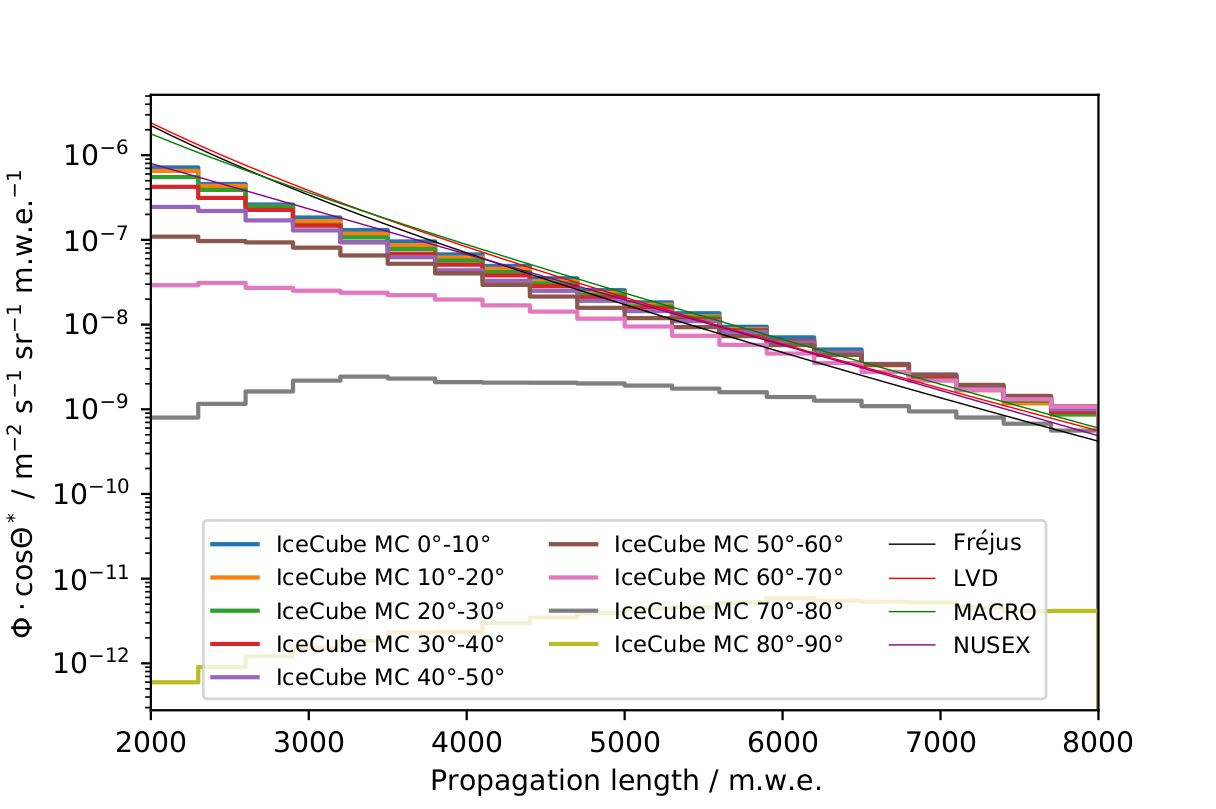
Fig. 40 : Muon depth intensity for different zenith intervals, calculated on the basis of generated MC events for the 20904 data set. This depth intensity has no connection to the event selection of the analysis and merely serves the purpose of reviewing the existing CORSIKA simulations. For comparison, the results of LVD, MACRO, Fréjus and NUSEX are shown (solid lines).

Another aspect is the propagation of muons through the ice, which is carried out using the lepton propagator PROPOSAL. For most of the existing simulations, the muon propagation behind the detector consist of a single continuous step (as shown in this config, where the configurations are explained here). This leads to the fact that muons with the same energy exiting the detector will travel the exact same distance from that point on. However, they should be propagated individually with the corresponding energy losses.

It is important to keep in mind that the muons propagate not just through the upper ice layers, but also through a bedrock layer that lies several hundred meters below the detector. PROPOSAL uses a model with the following specs:

Table 4 : PROPOSAL underground medium specs

Depth / m	Medium	Density / \(\frac{\mathrm{g}}{\mathrm{cm}^2}\)
< 200	Ice	0.7629
200 - 2810	Ice	0.9216
> 2810	Bedrock	2.65

New CORSIKA Simulations

The correct muon propagation is a rather simple task. PROPOSAL needs to be rerun with updated settings. Retrieving the muons that are cut out due to the energy cut is not possible using existing simulations. This is why we aim to generate new CORSIKA simulations in the corresponding energy range.

Creating new CORSIKA data without the angular dependent energy cut yields a much more plausible result (see Fig. 41) where the depth intensity for the different zenith intervals is in good agreement. The results are in line with the findings of the other experiments. However, there is a slight overestimation of muons with large propagation lengths.

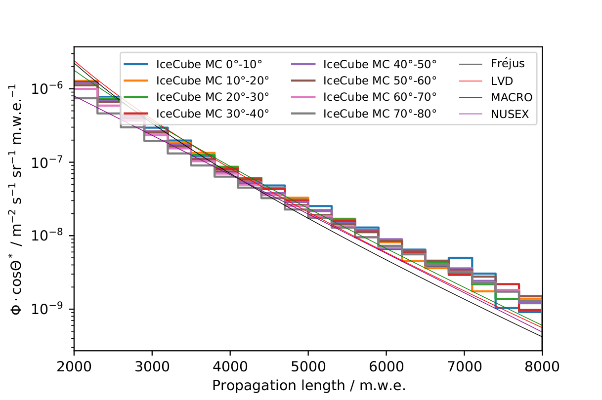
Fig. 41 : Muon depth intensity for different zenith intervals, calculated on the basis of generated MC events using the adjusted CORSIKA simulations. For comparison, the results of LVD, MACRO, Fréjus and NUSEX are shown (solid lines). The propagation length is converted to m.w.e., assuming a model as in Table 4.

The deviating shape is expected, as it results from the propagation through a different medium. For IceCube the detection medium is ice and not standardrock, as it is the case for the other experiments. This impacts the muons energy losses and results in the visible flattening. As a simple test, the same muons are propagated again, but this time through standardrock (using PROPOSAL with adjusted settings for the medium). The stopping muon depth intensity is determined following the same principle as before. The result is shown in Fig. 42, where the intensity is in even better agreement with the other experiments.

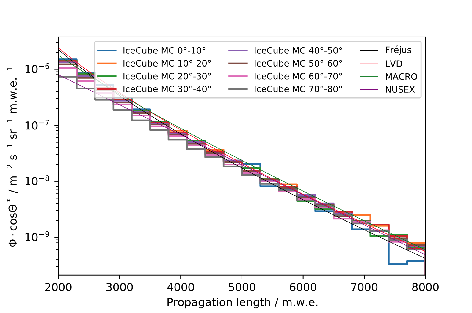
Fig. 42 : Muon depth intensity for different zenith intervals, calculated on the basis of generated MC events using the adjusted CORSIKA simulations and a propagation through standardrock. For comparison, the results of LVD, MACRO, Fréjus and NUSEX are shown (solid lines).

In summary, the simulation of new untriggered data with the correct settings shows that the calculation of proper effective areas is indeed possible. Since the 20904 data set is to be used in the analysis, we aim to resimulate parts of the untriggerd 20904 data to meet our requirements. This data does not yet exist, but it is being simulated right now. This is why the following results are produced using our self-simulated unteriggered data (57500/58500) for the moment. They should not change much depending on what data is used.