Results

Unfolding Results using funfolding

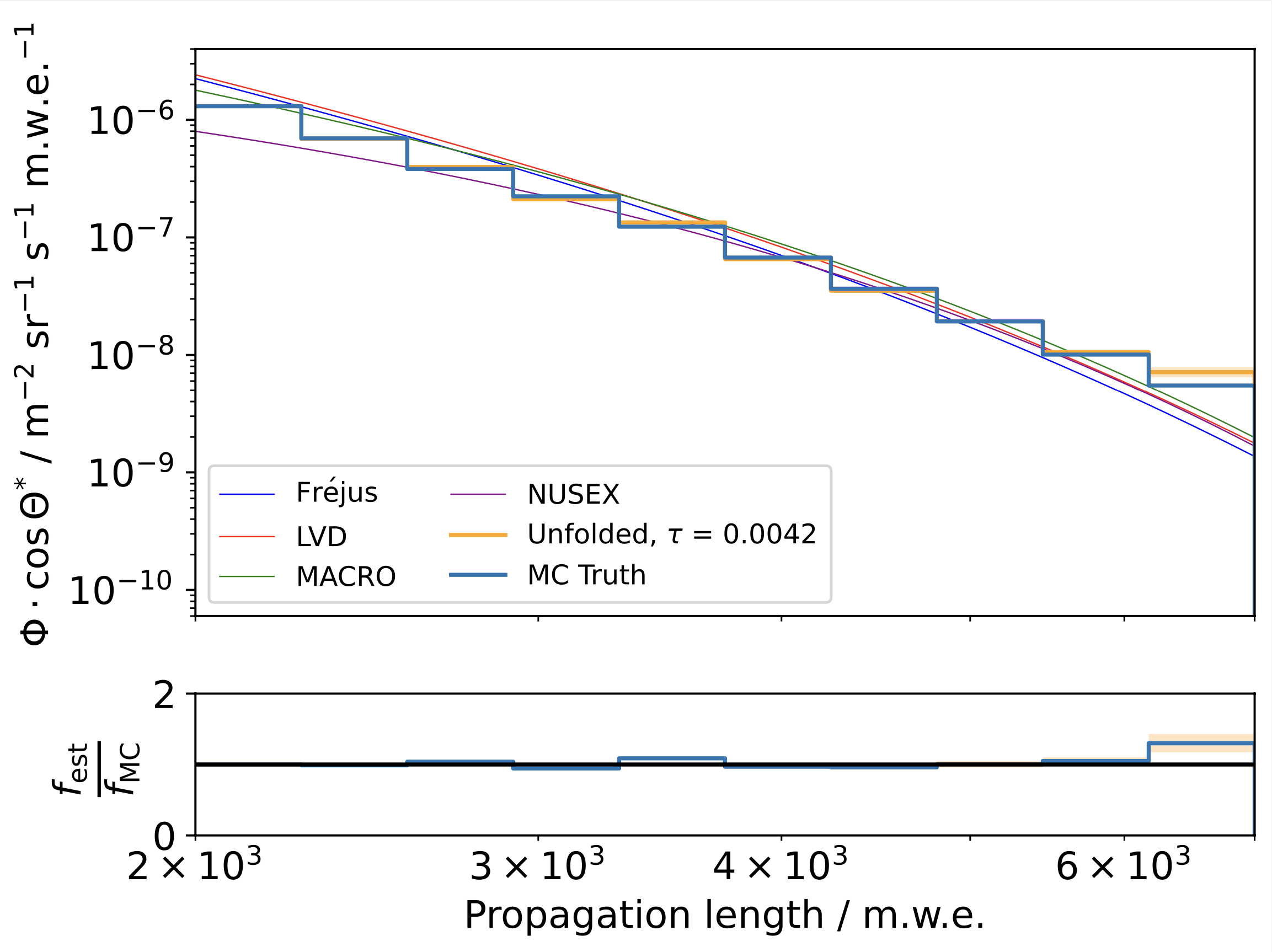
First unfolding results using funfolding are displayed below. Fig. 44 and Fig. 45 show the unfolded vertical stopping muon depth intensity with the two different effective area approaches from the Effective Area Estimation section. The latter is not being updated anymore and merely serves as a proof of concept. It shows that both effective area approaches yield almost identical results. The results are obtained on MC-data, using a training set of 300000 and a test set of 150000 events. The uncertainties are obtained using the MCMC approach. The plots only show statistical uncertainties since the 20904 snowstorm data is not yet available and it is not possible to unfold the whole target range with the limited snowstrom statistics that I simulated myself (more on that in the Systematic Checks section).

Fig. 44 : Top: Unfolded vertical stopping muon depth intensity using the general effective area approach. The true distribution, determined from the MC-truth is shown in blue. The unfolded distribution is shown in orange including. The best fits of LVD, MACRO, Fréjus and NUSEX are illustrated by the solid lines. Bottom: Ratio plot of the true and unfolded flux with the corresponding quantiles.

Fig. 45 : Unfolded vertical stopping muon depth intensity using the adjusted effective area approach. The outline is the same as in Fig. 44.

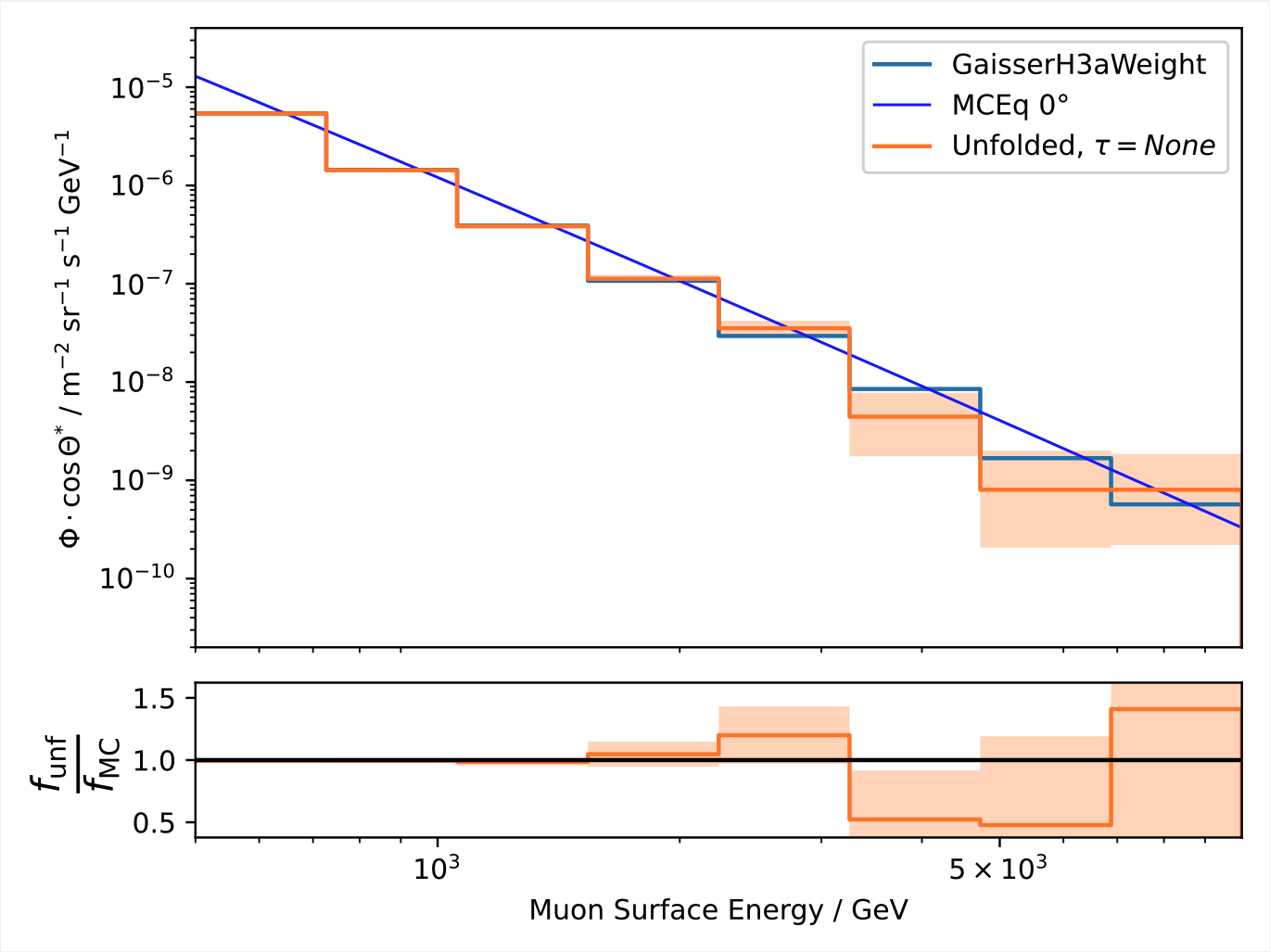
Fig. 46 shows the vertical muon surface energy spectrum in comparison with analytical MCEq results.

Fig. 46 : Unfolded surface energy spectrum in comparison with MCEq results.

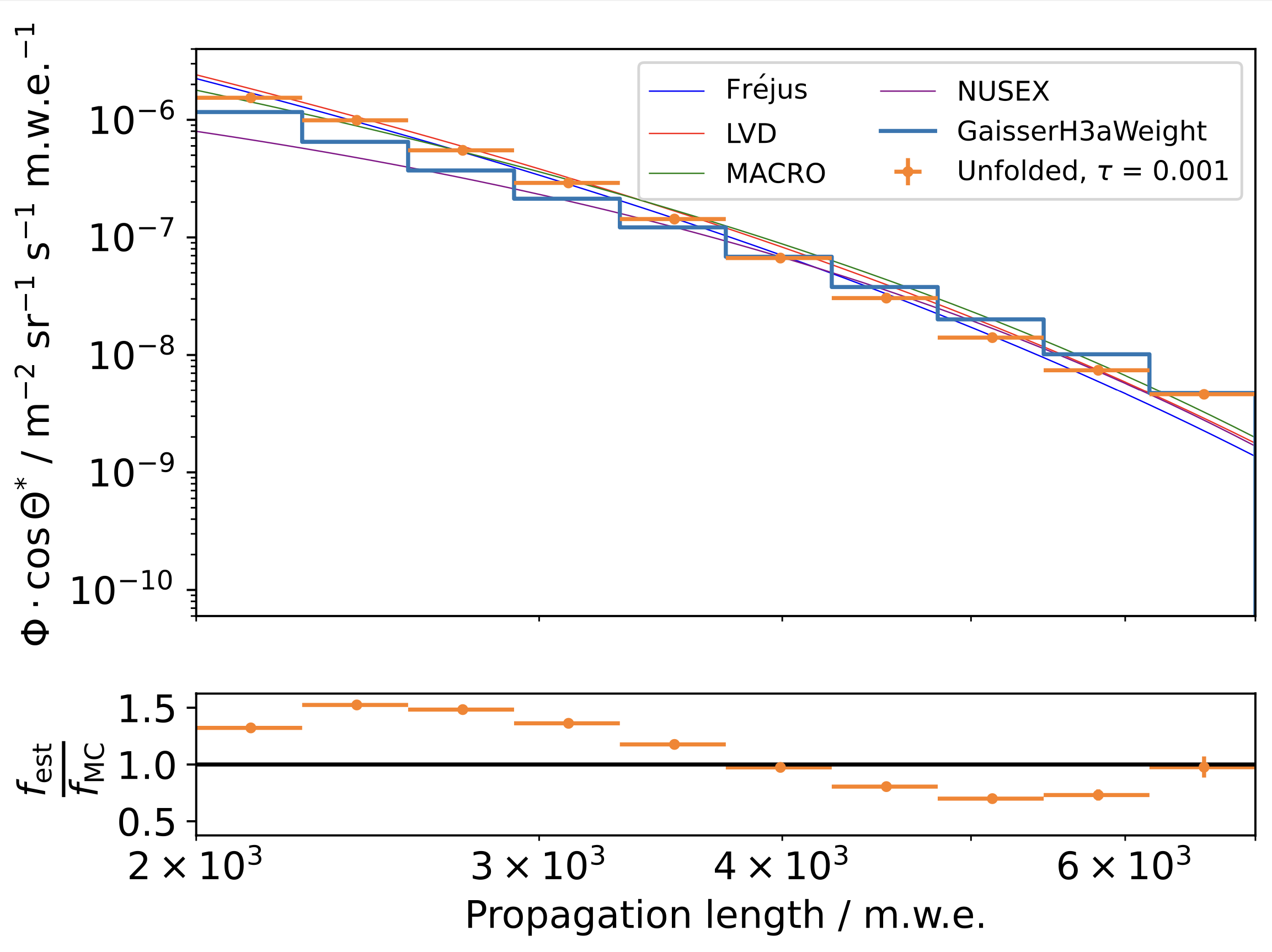
The results have also been determined on the mini-burnsample (see Table 3). The results are shown in Fig. 47 and Fig. 48.

Fig. 47 : Unfolded burnsample stopping muon depth intensity. The outline is the same as in Fig. 44.

Fig. 48 : Unfolded burnsample surface energy distribution. The outline is the same as in Fig. 46.