Unfolding

The Concept of Unfolding

The quantity of interest, the propagation length of the particles, is smeared out in the detection process due to the limited accuracy and sensitivity of the detector. Hence, it is impossible to determine the physical truth from the measurement directly. In fact, the measurement yields proxy variables, which stem from the detector response to the underlying physics. The inverse process, namely the determination of the most probable physical truth on the basis of the measurements, is referred to as unfolding.

The distribution of a measured quantity \(g(y)\) is connected to the true physical distribution \(f(x)\) via the detector response \(A(x,y)\) according to the convolution integral

\[\begin{equation} g(y) = \int A(x,y) f(x) \,\mathrm{d}x + b(y) + \epsilon(y) \; . \end{equation}\]

This is referred to as the Fredholm integral equation of the first kind. The additional term \(b(y)\) represents some bias, which originates form contributions to the measurement that are considered as background. Since the selected sample is assumed to have a sufficiently high purity, the bias will be neglected in the following. The quantity \(\epsilon(y)\) denotes systematic uncertainties, which are not yet taken into account. The detector response function \(A(x,y)\) describes the whole detection procedure. It depends on the physical truth and has to be determined from Monte Carlo simulations.

In practice, it is necessary to discretize the phase space of the variables \(x\) and \(y\). The integral has to be transformed into a sum

\[\begin{equation} g_{i} = \sum_{j} A_{ij} f_{j} \qquad \Rightarrow \qquad \textbf{g} = \textbf{A} \cdot \textbf{f} \; , \end{equation}\]

where the equation on the right represents a matrix multiplication with the detector response matrix \(\textbf{A}\) and the vectors \(\textbf{g}\) and \(\textbf{f}\). Each vector component denotes a bin entry in the distribution of the corresponding quantity.

Fig. 43 : Schematic representation of unfolding. The underlying physical truth is smeared in the detection process. This is described by the detector response \(A\). The inverse process, which determines the most probable physical truth on the basis of the measurements, is called unfolding.

The main task is the reconstruction of the true distribution \(\textbf{f}\) from the measured distribution \(\textbf{g}\). In principle, this could be done by simply inverting the discrete Fredholm equation. However, the response matrix is not necessarily a square matrix and even if the inverse \(\textbf{A}^{-1}\) exists, the solution often shows an oscillating behavior. This would be an unphysical result and can be traced back to the properties of the matrix itself. The approach is an ill-posed problem, where small eigenvalues of the matrix heavily amplify statistical noise in the measurement. Consequently, more sophisticated methods are needed to unfold the true spectrum.

Maximum Likelihood Estimation

One such approach is a maximum likelihood estimation. A likelihood function is constructed by assuming a Poisson distribution for each bin of the proxy variable

\[\begin{equation} \mathcal{L}(\textbf{g}|\textbf{f}\,) = \prod_{i} \frac{\lambda_{i}(\textbf{f}\,)^{g_{i}}}{g_{i}!} \exp{\left(-\lambda_{i}(\textbf{f}\,)\right)} \; , \end{equation}\]

where the used model \(\lambda_{i}(\textbf{f}\,)\) corresponds to the discrete Fredholm equation

\[\begin{equation} \mathcal{L}(\textbf{g}|\textbf{f}\,)= \prod_{i} \frac{(\textbf{A} \cdot \textbf{f}\,)_{i}^{g_{i}}}{g_{i}!} \exp{\left(-(\textbf{A} \cdot \textbf{f}\,)_{i}\right)} \; . \end{equation}\]

The most probable distribution \(\textbf{f}\) on the basis of the measurements \(\textbf{g}\) maximizes the likelihood. For practical reasons, it is often useful to minimize the negative logarithm of this function instead. The result remains unchanged, but the likelihood reads

\[\begin{equation} l(\textbf{g}|\textbf{f}\,) = \sum_{i} \Big((\textbf{A} \cdot \textbf{f}\,)_{i} - g_{i} \ln{\left((\textbf{A} \cdot \textbf{f}\,)_{i}\right)}\Big) \; , \end{equation}\]

The complication of oscillating solutions still remains. To overcome this problem, it is necessary to introduce additional assumptions about the smoothness of the distribution. This method is referred to as regularization. A commonly used form of regularization is the Tikhonov regularization. It introduces a penalty term which suppresses high second derivatives of the solution

\[\begin{equation} \mathcal{R}(\textbf{f}\,) = \frac{1}{2} \tau^{-1} \, \textbf{f}^{T} \, \textbf{C}^{T} \, \textbf{C} \, \textbf{f} \; , \end{equation}\]

with the regularization matrix

\[\begin{split}\begin{align} C = \begin{bmatrix} -1 & 1 & 0 & & \dots & & 0 \\ 1 & -2 & 1 & & & & \\ 0 & 1 & -2 & & & & \vdots \\ & & & \ddots & & & \\ \vdots & & & & -2 & 1 & 0 \\ & & & & 1 & -2 & 1 \\ 0 & & \dots & & 0 & 1 & -1 \\ \end{bmatrix} \; . \end{align}\end{split}\]

It is chosen such that \(\textbf{C} \textbf{f}\) is the second derivative according to the finite difference method. The parameter \(\tau\) controls the strength of the regularization. Introducing a regularization serves as a form of bias. It is important to optimize its strength in such a way that the oscillations are suppressed, but the spectrum is not flattened to an extent that makes the result physically unreliable. The total likelihood then reads

\[\begin{equation} l(\textbf{g}|\textbf{f}\,) = \sum_{i} \Big((\textbf{A} \cdot \textbf{f}\,)_{i} - g_{i} \ln{\left((\textbf{A} \cdot \textbf{f}\,)_{i}\right)}\Big) + \frac{1}{2} \tau^{-1} \, \left(\textbf{C} \, \textbf{f}\right)^{T} \, \textbf{C} \, \textbf{f}\; . \end{equation}\]

Since bins of the target distribution \(\textbf{f}\) can be empty and the logarithm of zero is not definded, a small offset \(d\) is added. The target distribution is further subject to the detector response, which is why not \(\textbf{f}\) itself, but the logarithm of the acceptance corrected spectrum is expected to be flat. Hence, the regularization term is modified:

\[\begin{split}\begin{align} l(\textbf{g}|\textbf{f}\,) = &\sum_{i} \Big((\textbf{A} \cdot \textbf{f}\,)_{i} - g_{i} \ln{\left((\textbf{A} \cdot \textbf{f}\,)_{i}\right)}\Big) \\ &+ \frac{1}{2} \tau^{-1} \, \log_{10}{\left(A_{\mathrm{eff}}^{-1} \left(\textbf{f}+d \cdot \textbf{1} \right) \right)}^{T} \, \textbf{C}^2 \, \log_{10}{\left(A_{\mathrm{eff}}^{-1} \left(\textbf{f}+d \cdot \textbf{1} \right) \right)} \; . \end{align}\end{split}\]

funfolding

The concepts of ML unfolding have already been implemented in a python package by Mathis Börner, a former member of the TU Dortmund group. The package is available via pip install funfolding. In addition to the above mentioned unfolding approach, the package features tools such as an MCMC sampling or the possibility of fitting nuisance parameters to the distributions, which improves the estimation of systematic uncertainties in the analysis. Funfolding has also been used in an earlier IceCube analysis (3yr NuMu analysis) where additional informaiton can be found.

MCMC Sampling

Funfolding evaluates the likelihood in a bayesian approach. A Markov Chain Monte Carlo (MCMC) sampling is used to contruct an a-posteriori distribution of the form

\[\begin{equation} p(\textbf{f}|\textbf{g}\,) = \frac{\mathcal{L}(\textbf{g}|\textbf{f}\,) \cdot p(\textbf{f})}{p(\textbf{g})} \; , \end{equation}\]

where the a-priori distribution of \(\textbf{f}\) is set to be uniform

\[\begin{split}\begin{align} p(f_{i}) = \begin{cases} \frac{1}{N} \quad \mathrm{for} \quad 0 \leq f_{i} \leq N \; , \\ 0 \quad \mathrm{else} \; . \end{cases} \end{align}\end{split}\]

The drawn samples depend only on the one sampled before them, and they are independent of all others. Starting from a random guess, the chain moves to another point by adding a noise from a predetermined distribution. The jump is accepted with a certain probability, following the concepts of a modified Metropolis-Hastings algorithm as implemented in the \(\texttt{EnsembleSampler}\) of the \(\texttt{emcee}\) python package. The new point is included in the sample.

Parameter Optimization

The regularization strength \(\tau\) and the log-offset \(d\) have to be optimized. This is done by means of a simple grid search which aims to minimize the chi-squared distance between the unfolded result (on MC data) and the MC truth. The following metric is calculated for the individual unfoldings:

\[\begin{equation} \chi^2 = \sum_\limits{i} \frac{(f_{\mathrm{true},i} - f_{\mathrm{unf},i})^2}{\sigma_{\mathrm{unf},i}^2} \end{equation}\]

Systematic Uncertainties

Certain parameters in the simulation chain have uncertainties, which is why it is necessary to estimate their impact on the analysis as so-called systematic uncertainties. In terms of unfolding, the systematics are described by systematic parameters, which are fitted to the data as additional nuisance parameters. The detector repsonse matrix then depends on these additional parameters:

\[\begin{equation} \textbf{A} \rightarrow \textbf{A}(\vec{\xi}\,) \end{equation}\]

For each systematic, new simulation sets are used. These simulation sets are created with the systematic parameters variing within their defined range. This enables to construct weighting functions \(\omega_{i}(\xi_{j})\) (\(i\): Bin, \(j\): Systematic) that present the relative change of the bin content compared to the baseline simulation. To consider all parameters in a single bin, the functions are multiplied

\[\begin{equation} \omega_{i}(\vec{\xi}\,) = \prod_{j} \omega_{i}(\xi_{j}) \; . \end{equation}\]

The response matrix is then calculated as

\[\begin{equation} \textbf{A}(\vec{\xi}\,) = \mathrm{Diag}(\vec{\omega}(\vec{\xi}\,)) \, \textbf{A} \, . \end{equation}\]

The likelihood \(\mathcal{L}\) now also depends on the nuisance parameters \(\vec{\xi}\), which makes it possible to fit these parameters in the unfolding.

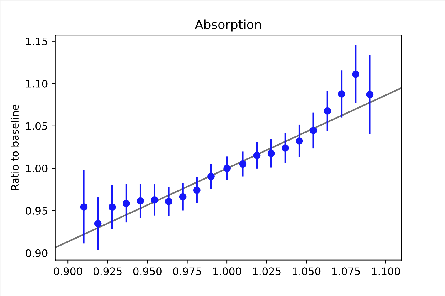
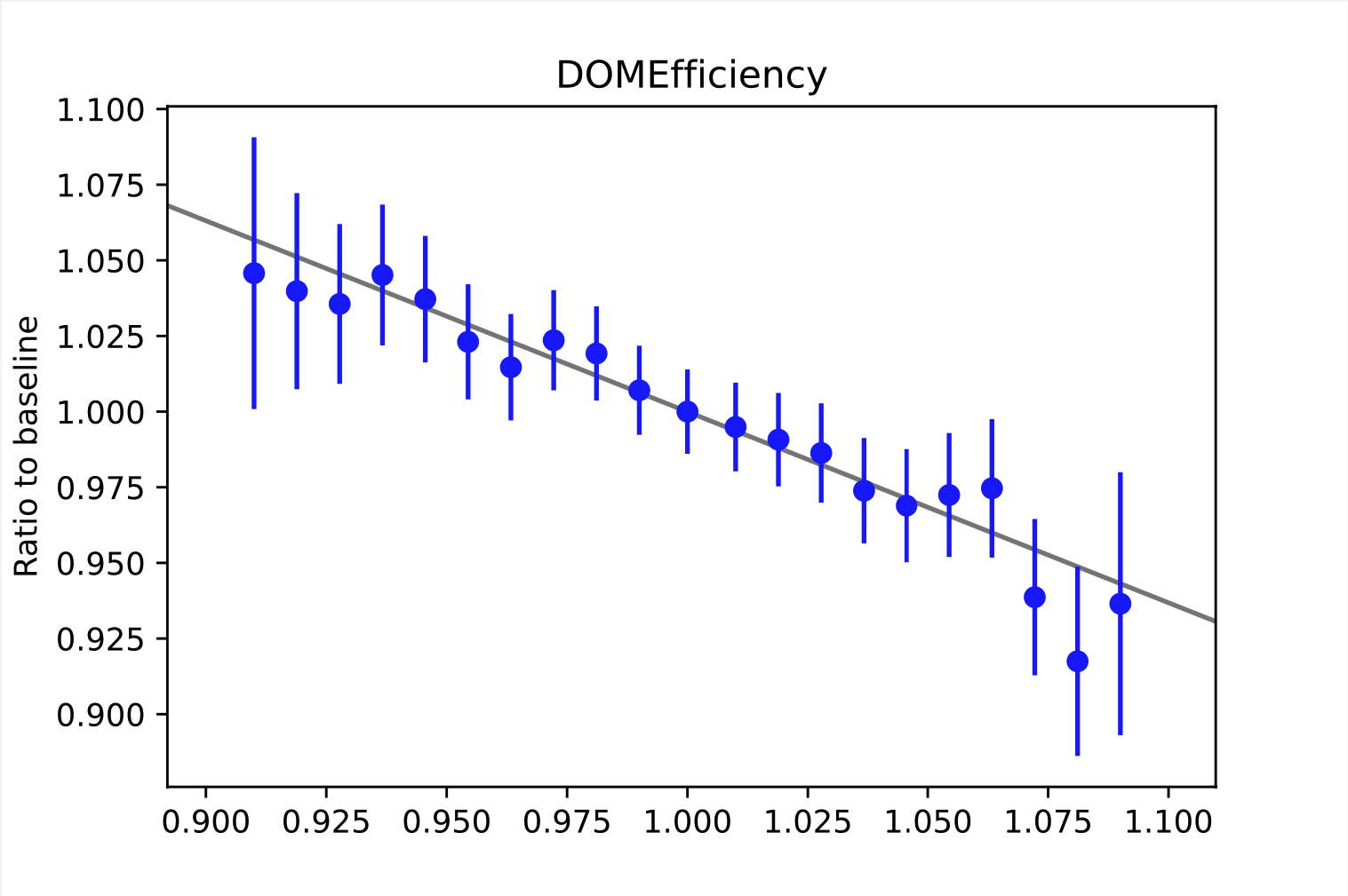
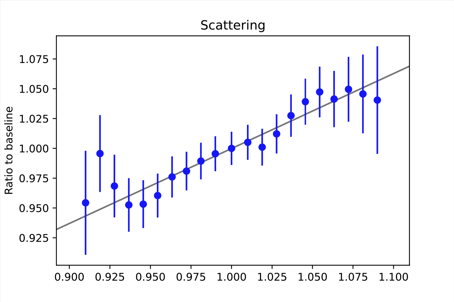
Some examples of weighting functions are shown below. As mentioned above, the weighting functions describe the relative change of the bin content. This refers to the bins of the observable space. Here, the examples are taken from random bins in the depth intensity unfolding, so they describe the change in the MC distribution (y-axis) based on the choice of the systematic parameters (x-axis). For energy unfolding, the concept remains the same. The baseline value for the systematic parameter depends on the exact systematic that is to be described. The baseline value always corresponds to the point where the ratio equals one. In order to interpolate between the data points, the ratio is fitted. The resulting function resemples the weighting function \(\omega_{i}(\xi_{j})\).

It is necessary to determine these ratios on MC data, since the information about the change of the true target quantity is needed. As far as we know, there are no systematic data sets for the 20904 set. Thus, we used our self-simulated data (58500/57500, see Table 2) that was simulated with snowstorm to construct the weighting functions. An advantage of snowstorm simulations is the possibility of creating a wide range of grid points, making the description more accurate.

All systematics, except for the second HoleIce parameter, can be fitted with a linear funciton.

In additon to the in-ice systematics we also consider the impact different flux models. Further details about their impact are discussed in the Systematic Checks section.