Event Selection

The analysis is conducted on an event sample of stopping atmospheric muons. These particles enter the antarctic ice sheet and stop inside IceCube’s detection volume due to a complete energy loss or decay. Their track signature in the detector enables the reconstruction of the stopping point and arrival direction. The classification and reconstruction tasks are performed by a deep neural network, serving as a robust method with a comparably short runtime.

Data Sets

The analysis requires labeled Monte Carlo data to train the network, but also to estimate the detector response matrix in the unfolding procedure and to assess the detection probability of stopping muons in the detector. Level 2 data is chosen as a starting point for the analysis. Although IceCube provides higher processing levels, many stopping muon events are assumed to be cut out in further processing steps, since these events are not necessarily well reconstructable (low energy events with short tracks in the detector). At level 2, most of the events are still in the sample. The FSSFilter is selected as filter stream for the analysis. This choice will be motivated further below.

The estimation of the detection probability (effective area) leads to an additional requirement: Knowledge about the initially generated events (pre-trigger level). A data set that fulfills all these requirements is the 20904 set. Further details are listed in Table 1.

Table 1 : Monte Carlo data set details

ID Number	Year	Primary Energy	Angular Range	Spectral Index
20904	2020	\(600\) GeV - \(10^{8}\) GeV	\(0\) ° - \(89.99\) °	\(-2\)

However, using the 20904 data set appears to be problematic for reasons described in the following section. This is why two new CORSIKA data sets are created to cover a sufficient range in energy. Details about these sets are listed in Table 2.

Table 2 : New CORSIKA data set details

ID Number (unofficial)	Year	Primary Energy	Angular Range	Spectral Index
58500	2022	\(100\) GeV - \(10^{5}\) GeV	\(0\) ° - \(89.99\) °	\(-2\)
57500	2022	\(10^{5}\) GeV - \(10^{8}\) GeV	\(0\) ° - \(89.99\) °	\(-2\)

The number of events on Level 2 is 667517.

The MCs are subsequently weighted to the GaisserH3a-model. Using a different model should impact the distributions of energy and propagation length to a certain extend. However, the unfolding procedure should in principle be very robust/independent of the used flux model. Further checks are provided in the unfolding section.

The scripts and the Data-MC agreement of the reconstructions are usually tested on a 1% burn sample. Since the event rate of atmospheric muons is very high, these tests have been performed on only about 20 minutes of data so far. The data is taken from different days over the year to account for seasonal variations. Details in Table 3.

Table 3 : Measured data sets

Date	Total Runtime / s	Event Rate / Hz (Selection)
2020/XX/01 (XX = [06, 08, 12])	1206.10	50.25

We choose the FSSFilter as filter stream because it yields the highest event rate for low energy stopping muons. A comparison between different filter streams that yield a reasonable amout of statistics is shown in Fig. 3, where Fig. 4 shows the reconstruction quality of the muon propagation length. The reconstructed length is calculated based on the DNN output. This will be further explained below.

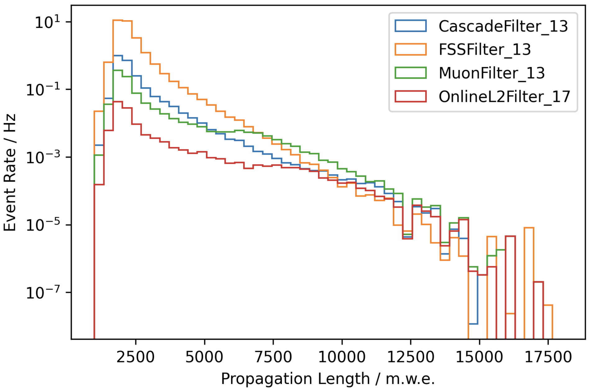
Fig. 3 : True Propagation length distribution for different filters.

Fig. 4 : Reconstruction error for different filters.

Deep Neural Network

The network estimates the following parameters for each event:

• Classification score

• Vertical stopping depth

• Direction

The confidence level of an event being a stopping event is quantified by assigning score values between zero and one. Events with a higher score have a larger probability to be a stopping event, whereas a low value is assigned to events that are most likely through-going and therefore considered as background. In addition, the network estimates the uncertainties of the reconstructed quantities per event based on an assumed Gaussian likelihood.

The DNN is trained on level 2 simulation data from the 20904 data set using the dnn_reco framework (documentation). Only three parameters are used as input:

• Total DOM charge (for each DOM individually)

• Relative time of first pulse (per DOM, relative to total time offset, calculated as the charge weighted mean time of all pulses)

• Charge weighted standard deviation of pulse arrival times (per DOM)

In order to use level 2 data as training data for the network, it has to be pre-processed to create to corresponding input parameters as well as the labels that it should learn to reconstruct. The procedure of creating the input parameters is described in much detail here, where the processing relies on pre-defined modules from the ic3-data repository. The exact module is:

from ic3_data.segments import CreateDNNData

tray.AddSegment(CreateDNNData, 'CreateDNNData',
                NumDataBins=3,
                RelativeTimeMethod='time_range',
                DataFormat='reduced_summary_statistics_data',
                PulseKey='CleanedMuonPulses')

The CleanedMuonPulses pulse series does not exist on level 2 data in the standard IceCube processing. It is additionally created using the following module, where the SplitInIcePulses already exist on level 2 data:

from icecube import DomTools

tray.AddModule('I3TimeWindowCleaning<I3RecoPulse>', 'TimeWindowCleaning',
               InputResponse = 'SplitInIcePulses',
               OutputResponse = 'CleanedMuonPulses',
               TimeWindow = 6000*icetray.I3Units.ns)

The labels are created using the modules from the stoppingmuons repo:

from processing_scripts.scripts.l2precuts.stopping_muon_mc_label import CreateStoppingMCLabels

tray.Add(CreateStoppingMCLabels, 'CreateStoppingMCLabels')

The training data does not require further processing and it can now be used to train the network.

Fig. 5 - Fig. 7 show the data-MC agreement of the input parameters. The distributions show the pulses of all DOMs together. The relative time is in quite good agreement, whereas there are slightly larger deviations visible in the total charge and the standard deviation of arrival times. The agreement for the charge gets worse for pulses with larger total charge. For the standard deviation of pulse times, there appears to be a region of increasing disagreement that subsequently reverses to a better agreement at larger values.

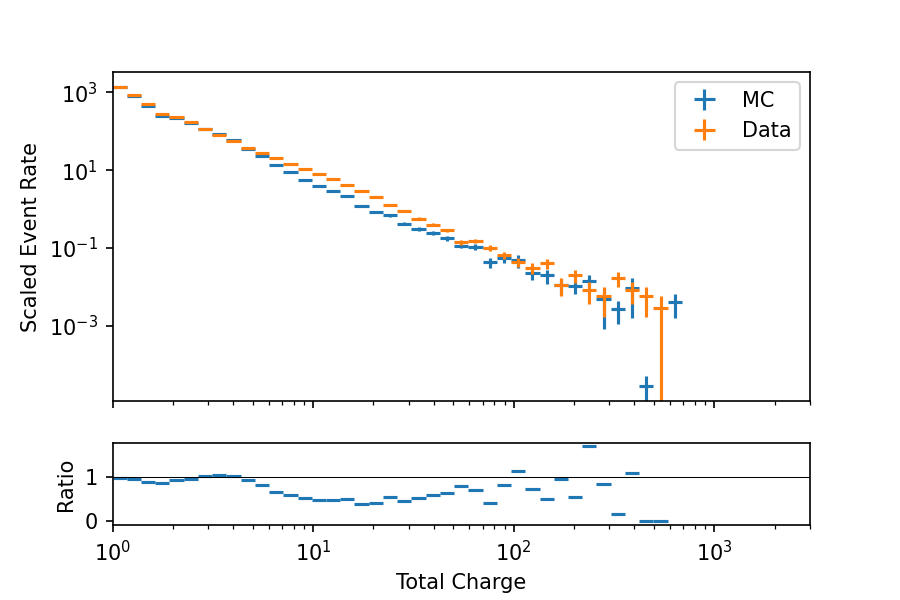
Fig. 5 : Data-MC agreement of total charge. The MC event rate is upscaled by 20%.

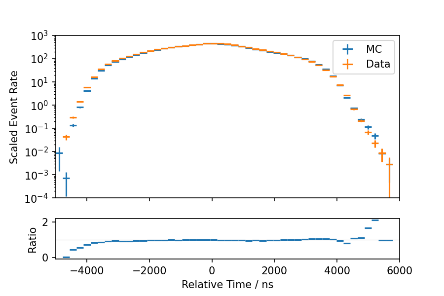
Fig. 6 : Data-MC agreement of relative time. The MC event rate is upscaled by 20%.

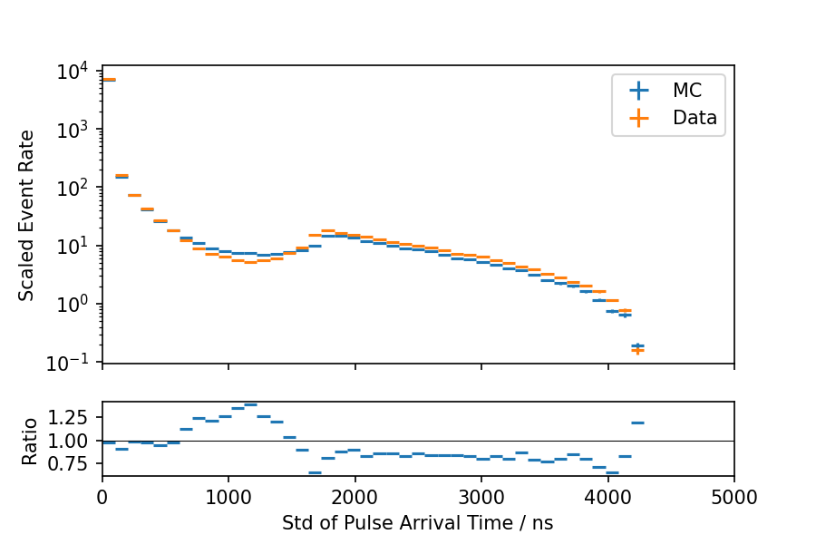
Fig. 7 : Data-MC agreement of charge weighted standard deviation of pulse arrival times. The MC event rate is upscaled by 20%.

The plots below show the agreement for other filtermasks. The MC rate is again upscaled by 20% in each plot.

MuonFilter:

CascadeFilter:

OnlineL2Filter:

The network’s robustness is further tested by modifying the pulse series of the MC data, resulting in deviating distributions of the input parameters.

As a first test, the highest charge DOMs of each event are discarded. The resulting inputs are again shown in Fig. 8 - Fig. 10, where the data distribtions remain unchanged. It is obvious that many higher energetic pulses are discarded due to the modification, whereas the time of the first pulse and the standard deviation of pulse times show minor differences.

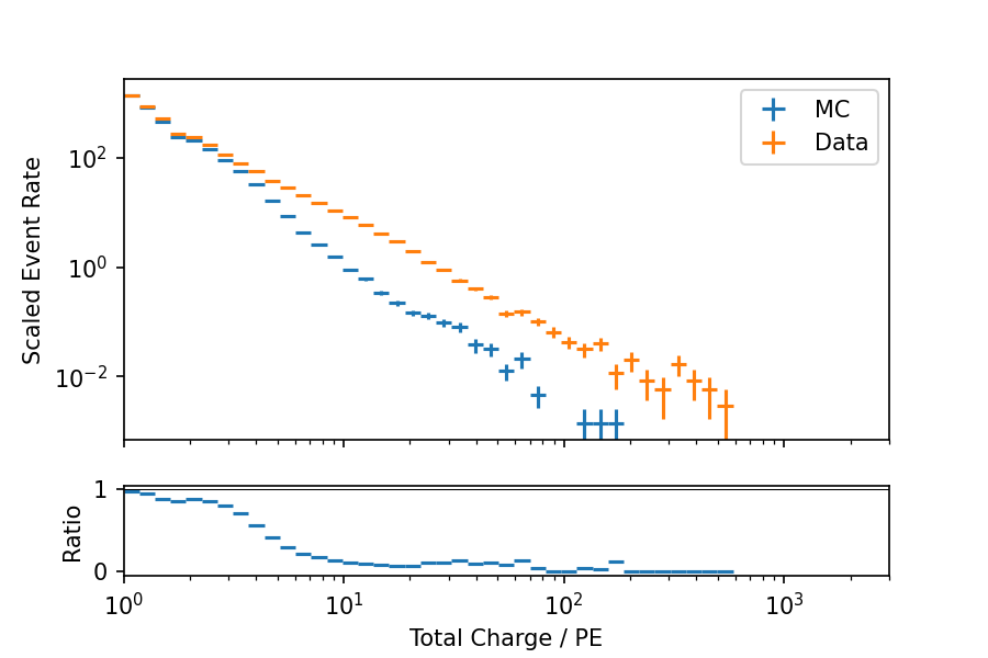
Fig. 8 : Data-MC agreement of total charge with modified MC pulses (discard highest charge DOMs). The MC event rate is upscaled by 20%.

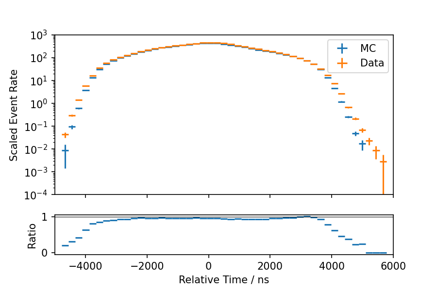
Fig. 9 : Data-MC agreement of relative time with modified MC pulses (discard highest charge DOMs). The MC event rate is upscaled by 20%.

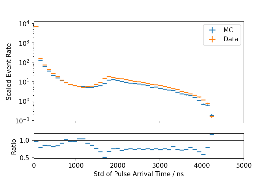
Fig. 10 : Data-MC agreement of charge weighted standard deviation of pulse arrival times with modified MC pulses (discard highest charge DOMs). The MC event rate is upscaled by 20%.

Fig. 11 and Fig. 12 show the differences of the stopping depth and zenith reconstructions on a per event basis (modified pulses compared to non-modified pulses). For the majority of events the reconstructions are barely affected. A few events tend to be reconstructed with a stopping depth closer to the surface for the modified pulses. This is expected since a muon track is more likely to be a little shorter in this case.

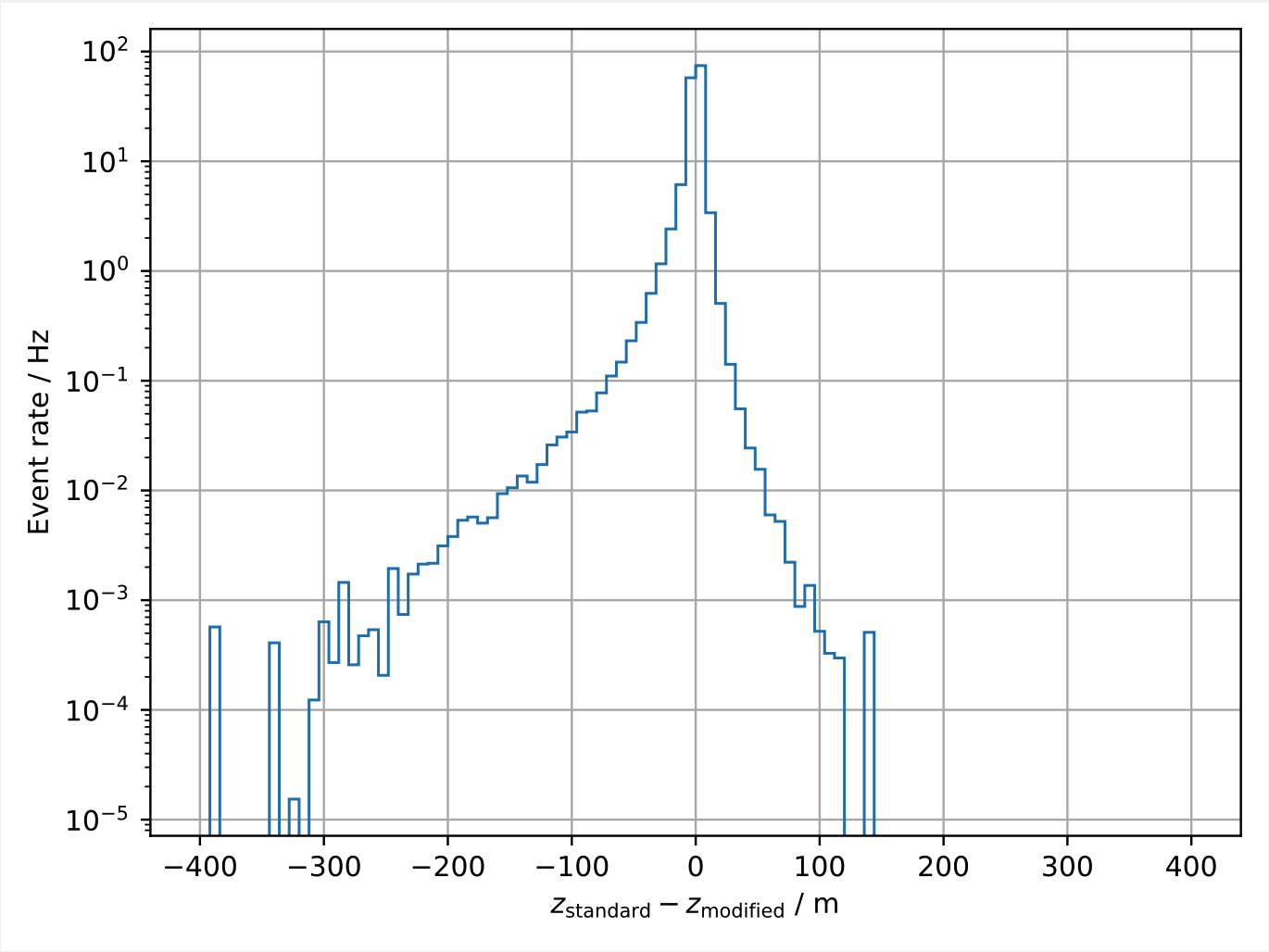
Fig. 11 : Per event differences of the stopping depth reconstructions with modified pulses compared to unmodified pulses. The pulses are modified by discarding the highest charge DOM of each event.

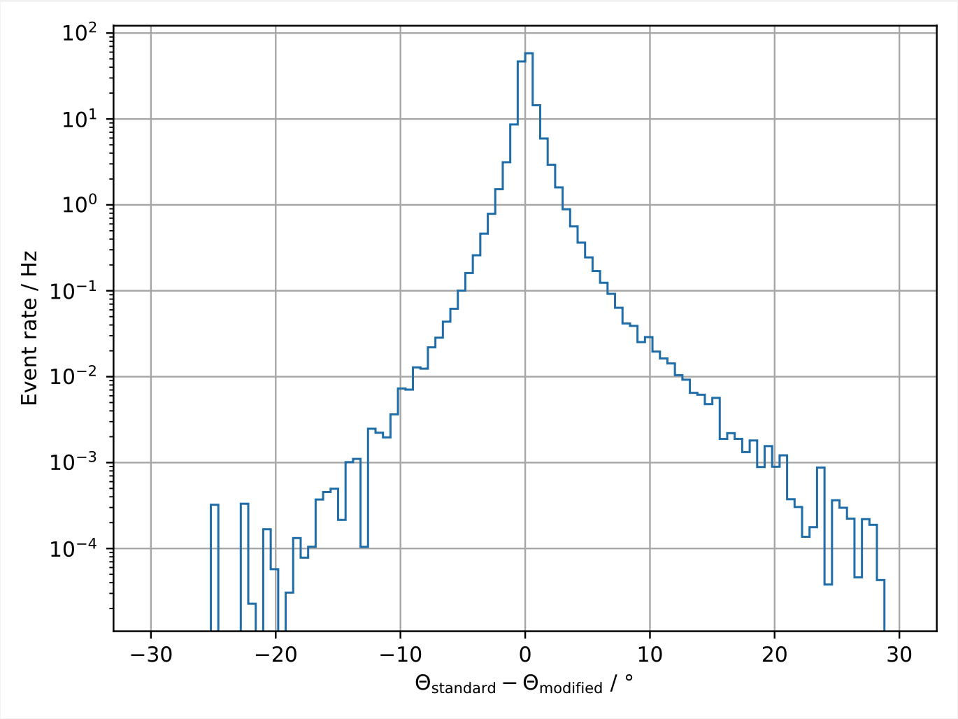
Fig. 12 : Per event differences of the zenith reconstructions with modified pulses compared to unmodified pulses. The pulses are modified by discarding the highest charge DOM of each event.

A similar test is performed by modifying the pulses in a way that random pulses are added to the pulse series. Fig. 13 - Fig. 15 show the input distributions for this test. The impact of this modification turns out to be not as drastic as in the first test, however there are larger differences in the standard deviation of pulse times.

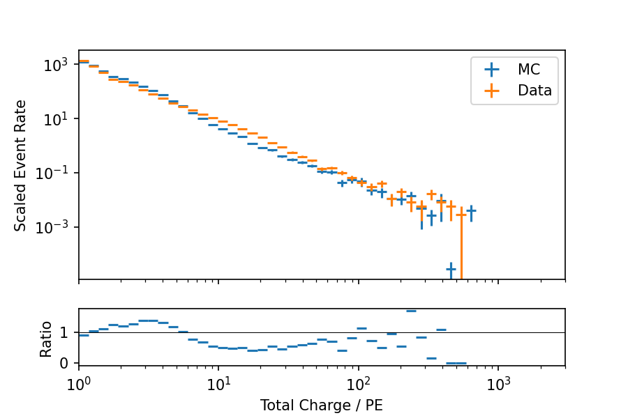
Fig. 13 : Data-MC agreement of total charge with modified MC pulses (discard highest charge DOMs). The MC event rate is upscaled by 20%.

Fig. 14 : Data-MC agreement of relative time with modified MC pulses (discard highest charge DOMs). The MC event rate is upscaled by 20%.

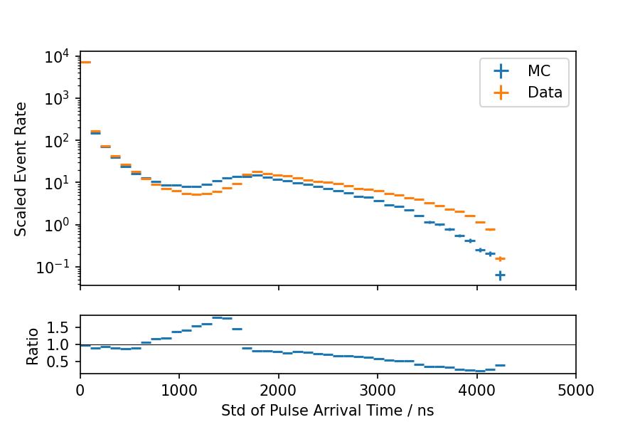
Fig. 15 : Data-MC agreement of charge weighted standard deviation of pulse arrival times with modified MC pulses (discard highest charge DOMs). The MC event rate is upscaled by 20%.

Fig. 16 and Fig. 17 again show the differences of the stopping depth and zenith reconstructions. There is now a bias towards an overestimation of the stopping depth since a muon track might seem longer if pulses are added. However, the effect is also much smaller.

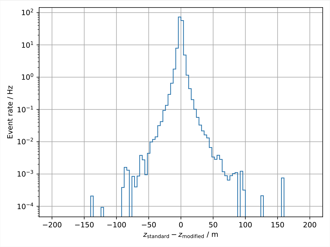
Fig. 16 : Per event differences of the stopping depth reconstructions with modified pulses compared to unmodified pulses. The pulses are modified by adding random pulses.

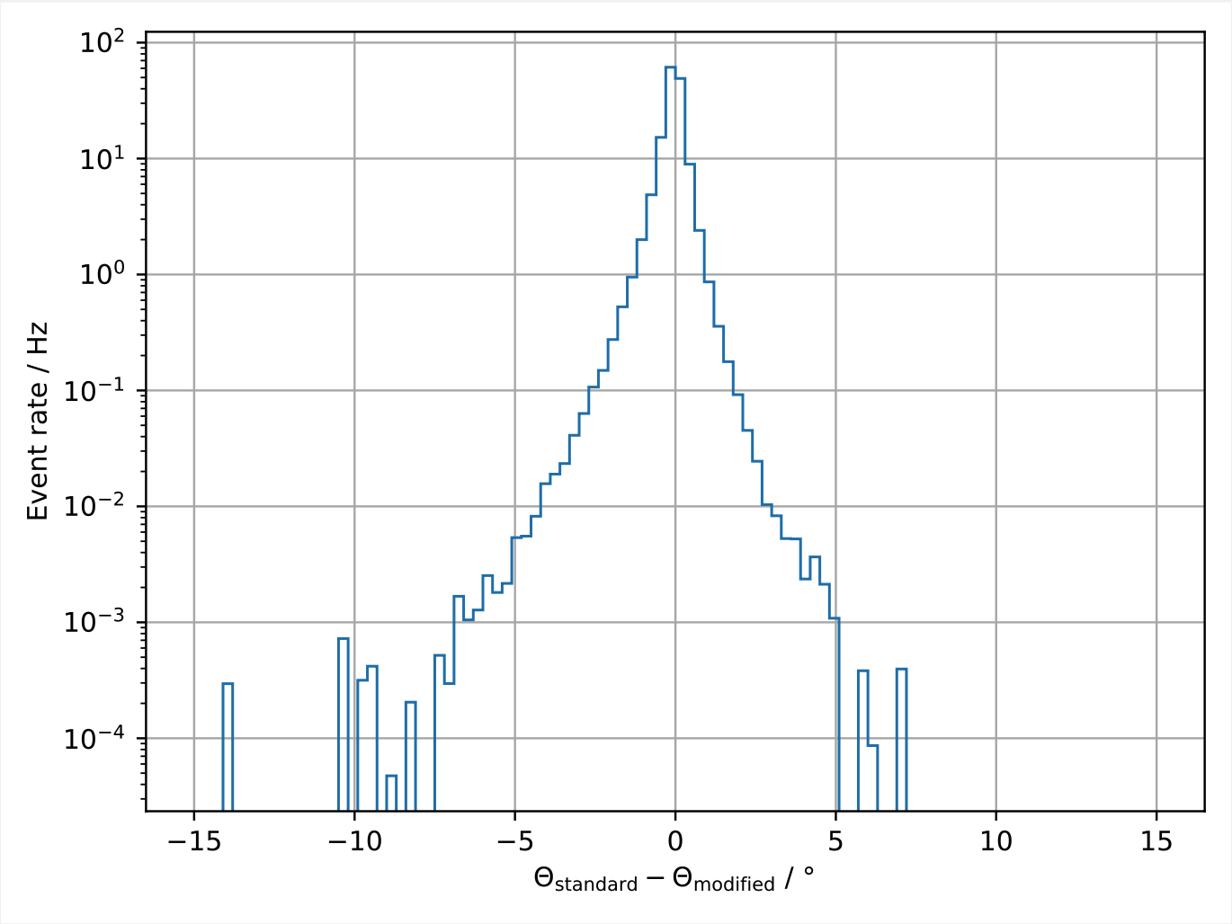
Fig. 17 : Per event differences of the zenith reconstructions with modified pulses compared to unmodified pulses. The pulses are modified by adding random pulses.

The required steps to run the DNN training are described in much detail in the Train Model section of the dnn_reco documentation. Note that the corresponding scripts are not included in this analysis repository. The config files with the used specifications to run the scripts will be provided in the Technical Documentation section.

The network adjusts its weights and biases according to a pre defined loss function. For the reconstruction tasks the network uses a Gaussian likelihood, whereas it uses MSE and cross entropy for the classification.

The classification and reconstructions are performed using three individual networks (one for each task). Each network uses the same architecture. They consist of a series of layers:

• 4 2D convolutional layers of upper DeepCore

• 8 2D convolutional layers of lower DeepCore

• 8 3D hexagonal convolutional layers over main IceCube array

• 1 fully connected layer

• Additional fully connected layer for uncertainty subnetwork

The performance of such a network has also been studied for the use of cascade reconstructions in the IceCube Neutrino Observatory.

Selection Results

Upon applying the DNN to the data, additional cuts are introduced on the estimated quantities to define the final selection results. It is further necessary to check the quality of the different reconstructions.

In order to select stopping muons, the most important estimation of the network is the score value. This value represents the network’s confidence of the corresponding event being a stopping muon event. An event with a score of 1 most likely corresponds to signal. The score distribution of the used CORSIKA data set is shown in Fig. 18.

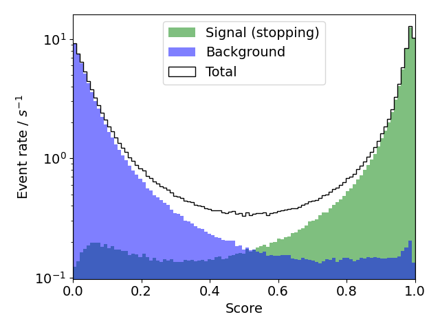
Fig. 18 : Score distribution, weighted to the GaisserH3a-model. The events are labeled regarding their MC-truth. Actual stopping events are marked green and background events are shown in blue. The network’s estimates are in good agreement with the MC-truth.

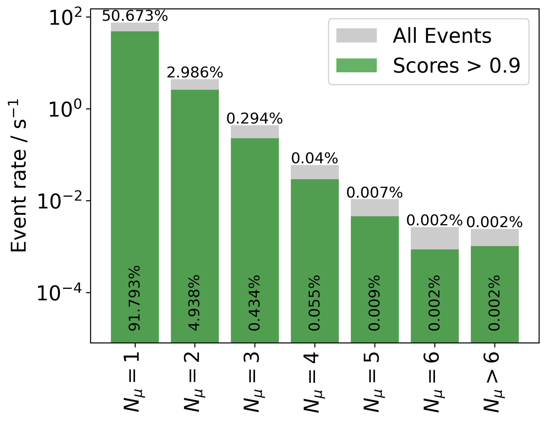
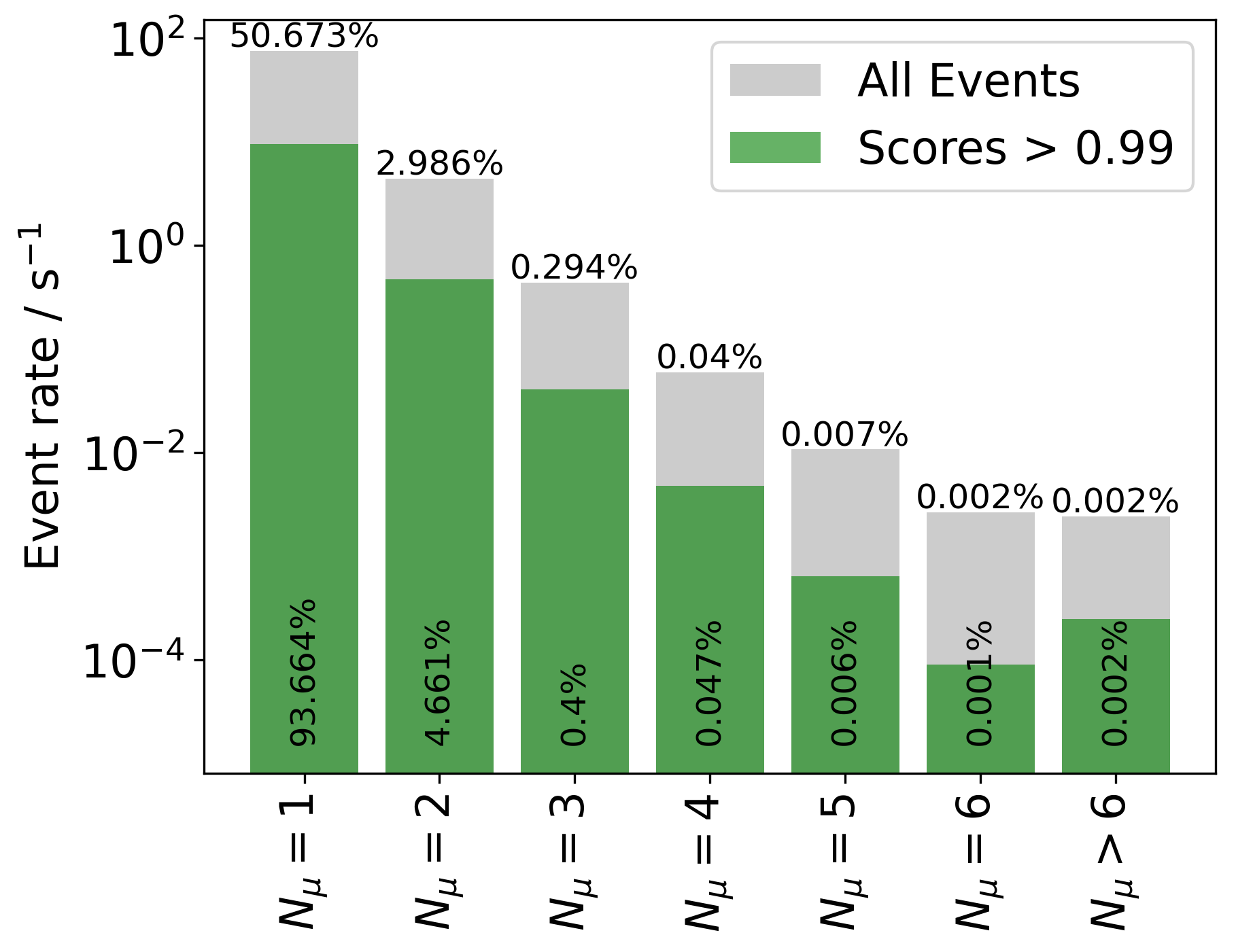
At this point it is also possible to check the initial assumption that most of the stopping muon events should be single muons. The plots below show the number of stopping muons in the detector for different score cuts in comparison to all events. For an increasing score cut, the percentage of single stopping muons increases. At a value of \(0.99\), over 90% of the selected events are single stopping muons. The percentages do not add up to 100% because there are also events without any stopping muon, which are not shown in these plots.

To determine appropriate cuts we aim to find a reasonable tradeoff between precision and recall. These quantities are defined by dividing the events into four groups:

• True positive (tp): A true stopping muon event is correctly classified as such.

• False positive (fp): A through-going event (background) is classified as a stopping event by the network.

• True negative (tn): A through-going event is correctly classified as such.

• False negative (fn): A true stopping muon event is classified as background.

The precision denotes the ratio of true stopping events in the final selection (tp) to all selected events (tp and fp):

\[\begin{equation} \mathrm{Precision} = \frac{\mathrm{tp}}{\mathrm{tp} + \mathrm{fp}} \end{equation}\]

The recall is the ratio of selected true stopping events (tp) to all simulated stopping events (tp and fn):

\[\begin{equation} \mathrm{Recall} = \frac{\mathrm{tp}}{\mathrm{tp} + \mathrm{fn}} \end{equation}\]

These two quantities are shown in Fig. 19 for different cuts on the score value. The shown precision as well as the high event rate of atmospheric muons motivate to apply a strict cut on the score value. It is not necessary to put a lot of emphasis on the recall, because even if there are a lot of muons cut out, there is still more than enough statistics to perform the analysis. The score cut is chosen to be

\[\begin{equation} \mathrm{Score} > \quad 0.99, \end{equation}\]

which serves as a reasonable tradeoff.

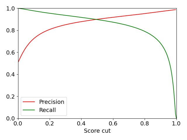
Fig. 19 : Precision and Efficiency of the classification for different cuts on the score value.

Introducing a cut on the score value is the most natural way of selecting stopping muon events from a set of data. Nevertheless, it is not the only estimation that is performed by the neural network. The precise determination of the stopping depth and the particle’s zenith angle is of equal importance to the inference of any physical result. The comparison of the estimated and true quantities is shown in Fig. 20 and Fig. 22 for the simple score cut. The network’s uncertainty estimations are shown as well in Fig. 21 and Fig. 23.

Fig. 20 : Comparison of estimated and true stopping depth with the score cut applied. The depth is shown in detector coordinates.

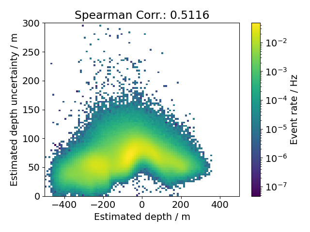
Fig. 21 : Estimated uncertainty of the stopping depth as predicted by the network.

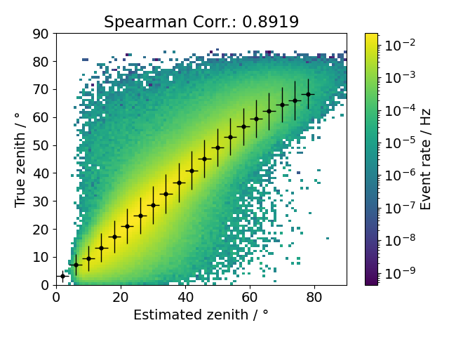
Fig. 22 : Comparison of estimated and true zenith angle with the score cut applied.

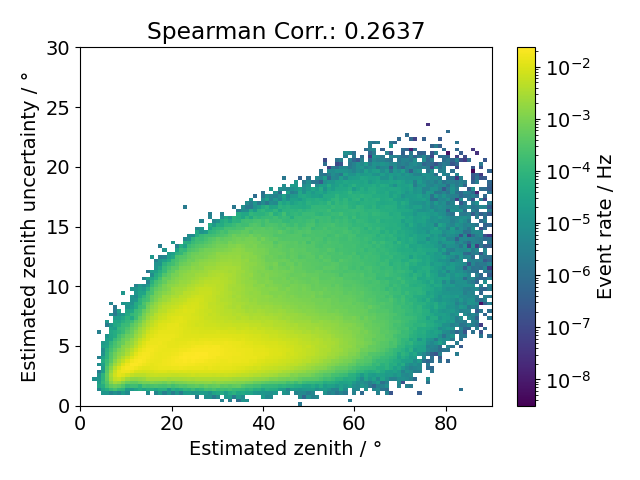
Fig. 23 : Estimated uncertainty of the zenith angle as predicted by the network.

It appears to be more difficult for the network to estimate the stopping depth around the center of the detector (\(0 \, \mathrm{m}\)). There are visibly more events deviating from the expected diagonal. This is also reflected in the depth uncertainty as it is larger for these events. So far we can not provide an explanation for why this is the case. In order to further improve the quality of the data set we aim to apply an additional cut on the depth uncertainty at \(60 \, \mathrm{m}\), cutting out the badly reconstructed events. Overall, the correlation is still quite high.

The zenith angle reconstruction performs even better in terms of the correlation. The figure also shows a certain amout of outliers, however there are no major misreconstructions. The uncertainty shows the largest pupulation of events below about \(6°\) over the whole zenith range. We focus on these better reconstructable events by applying an additional zenith uncertainty cut at \(0.1 \, \mathrm{rad}\). This cut is of course not as strongly motivated as the cut on the depth uncertainty and it is also expected to have less influence on the data set quality, but since there are no serious limitations in statistics we can safely choose these better reconstructable events for the stopping muon sample.

In summary, the final analysis cuts are definded as

\[\begin{split}\begin{align} &\mathrm{Score} &> \quad &0.99 \: &\cap \\ &\mathrm{Depth \: Unc.} &< \quad &60 \, \mathrm{m} \: &\cap \\ &\mathrm{Zenith \: Unc.} &< \quad &0.1 \, \mathrm{rad} \; &, \end{align}\end{split}\]

resulting in a precision of about 99%. The correlations of the final selection are shown in Fig. 24 and Fig. 25.

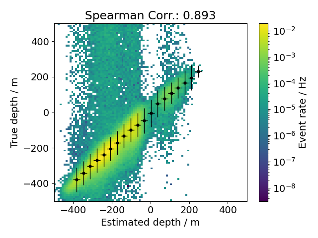
Fig. 24 : Comparison of estimated and true stopping depth with all analysis cuts applied.

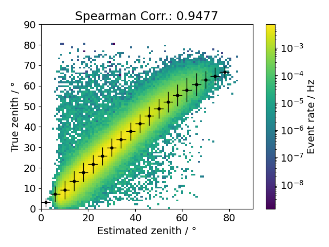
Fig. 25 : Comparison of estimated and true zenith angle with all analysis cuts applied.

The vertical stopping depth and the zenith angle of the muons are used to calculate the propagation length according to the equation in the previous section Ideally, the estimated stopping depth should correspond exactly to the underlying physical truth. However the propagation length does not totally agree with the MC-truth either. This is depicted in Fig. 26. It is expected to have a certain amount of misreconstructed events, since the whole precess of reconstruction is subject to the detector response. This is the motivation for applying an unfolding procedure.

Fig. 26 : Comparison of estimated and true propagation length with the score cut applied.

Since not just the stopping muon depth intensity, but also the surface energy spectrum is to be unfolded, the correlation of propagation length and muon surface energy is shown in Fig. 27.

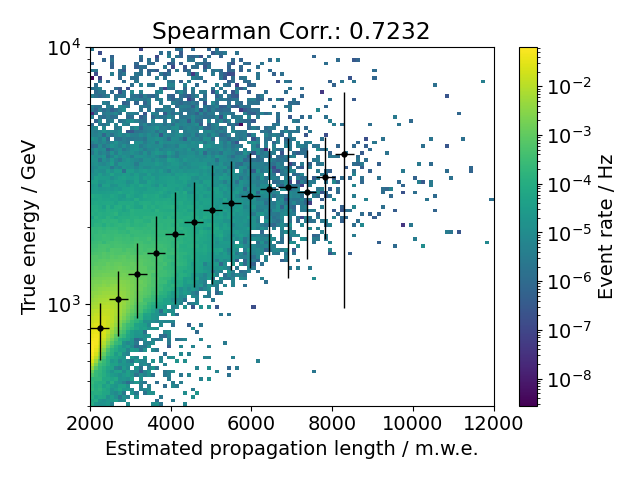
Fig. 27 : Comparison of estimated propagation length and true surface energy with the score cut applied.

Data-MC Agreement

It is important to assure the agreement of the reconstructions on simulation data with those on measured data. If the simulations would not describe the reality sufficiently well, any physical inference would be complicated. This is also crucial to the unfolding of the muon depth intensity, because it has to be trained on labeled data, even if applied to real measurements. The Data-MC agreement of all reconstructions is shown in Fig. 28 - Fig. 31.

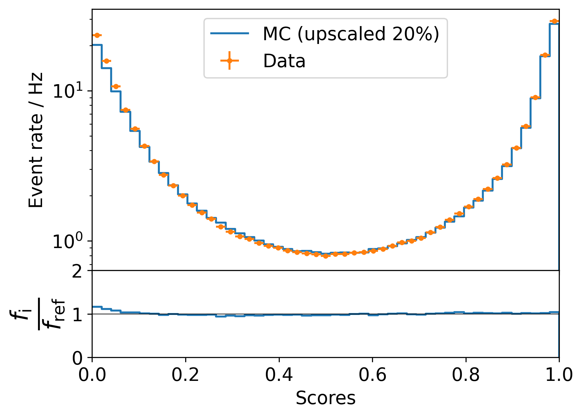
Fig. 28 : Data-MC agreement for the stopping muon scores (top). Ratio plot Data/MC (bottom).

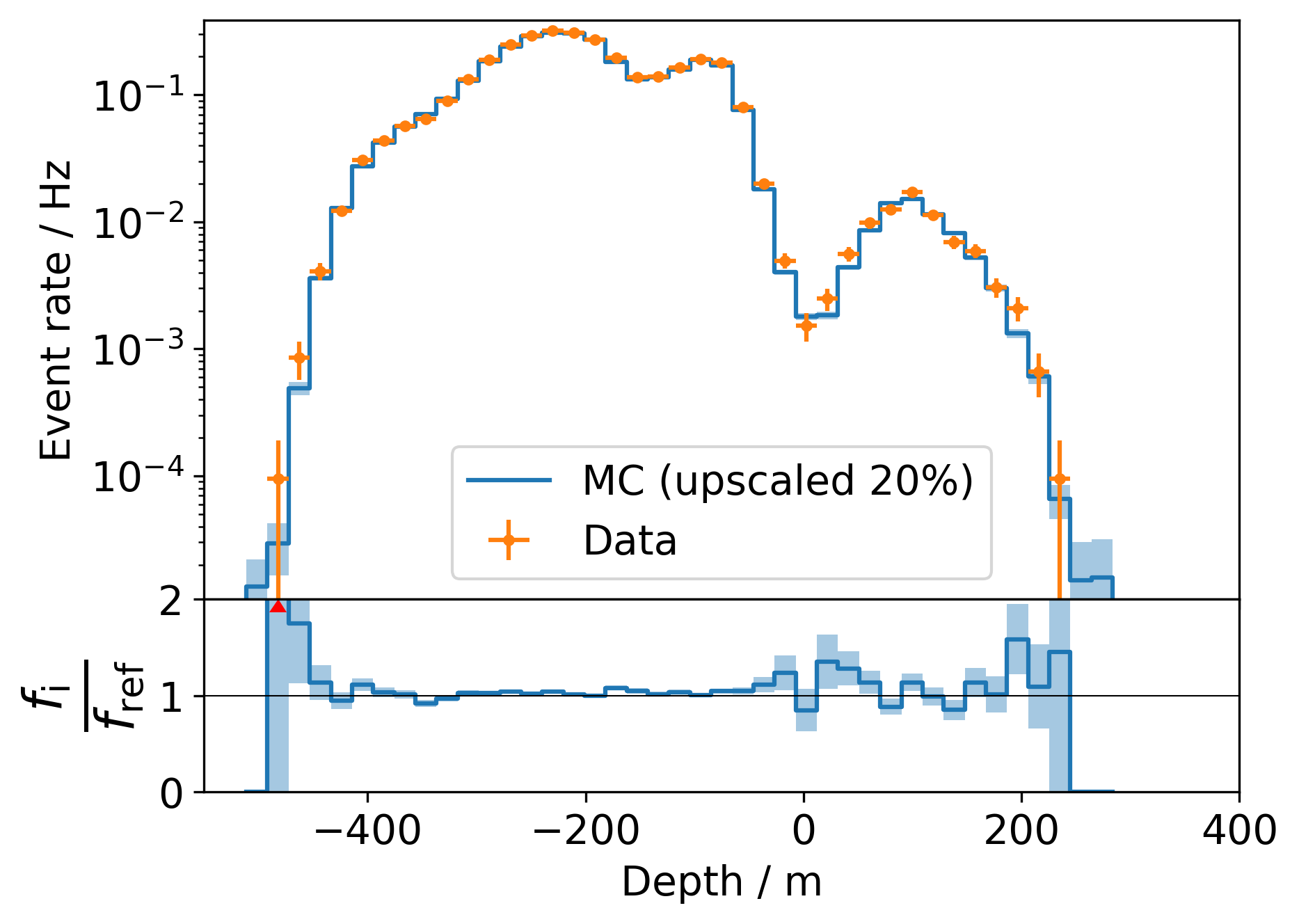
Fig. 29 : Data-MC agreement for the vertical stopping depth (top). Ratio plot Data/MC (bottom).

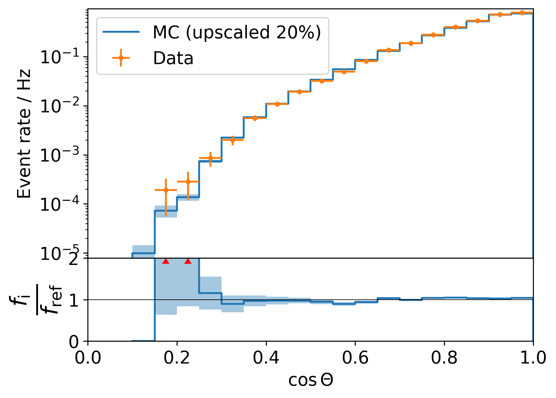
Fig. 30 : Data-MC agreement for the zenith angle (top). Ratio plot Data/MC (bottom).

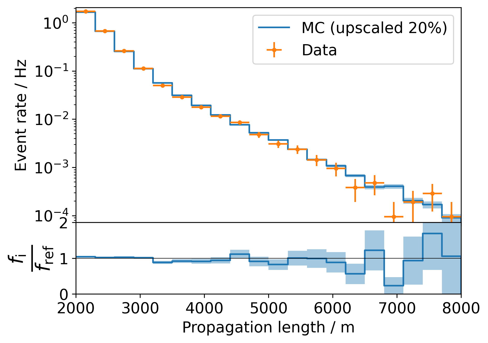
Fig. 31 : Data-MC agreement for the propagation length (top). Ratio plot Data/MC (bottom).

The scores, the stopping depth and the zenith show an offset of about 20% in data over MC, whereas the general shape is very similar. The offset itself is expected since we know that our simulations usually underestimate the number of muons by about 20%. Differences in the normalization do not have an impact on the unfolding. Events with low score predictions appear to be slighly overestimated for data compared to MC. The zenith shows a small transition to too many events at larger zeniths. We can not provide an explanation at this point, but a very similar behavior was found by Dennis in his paper (where the transition is much more prominent). There are also some deviations in the ratio of the propagation lengths for larger values, which seem to stem from limited statistics to a certain extend. Of course this should also have an impact on the unfolding results of data compared to MC. However, the whole concept of unfolding is meant to be very robust against such changes in the specturm. Further details are provided in the Unfolding section.

The same distribtions are again shown in Fig. 32 - Fig. 34 with a stricter score cut at 0.995:

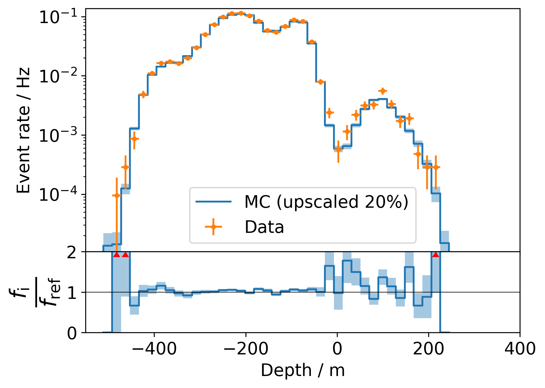
Fig. 32 : Data-MC agreement for the vertical stopping depth with a score cut at 0.995 (top). Ratio plot Data/MC (bottom).

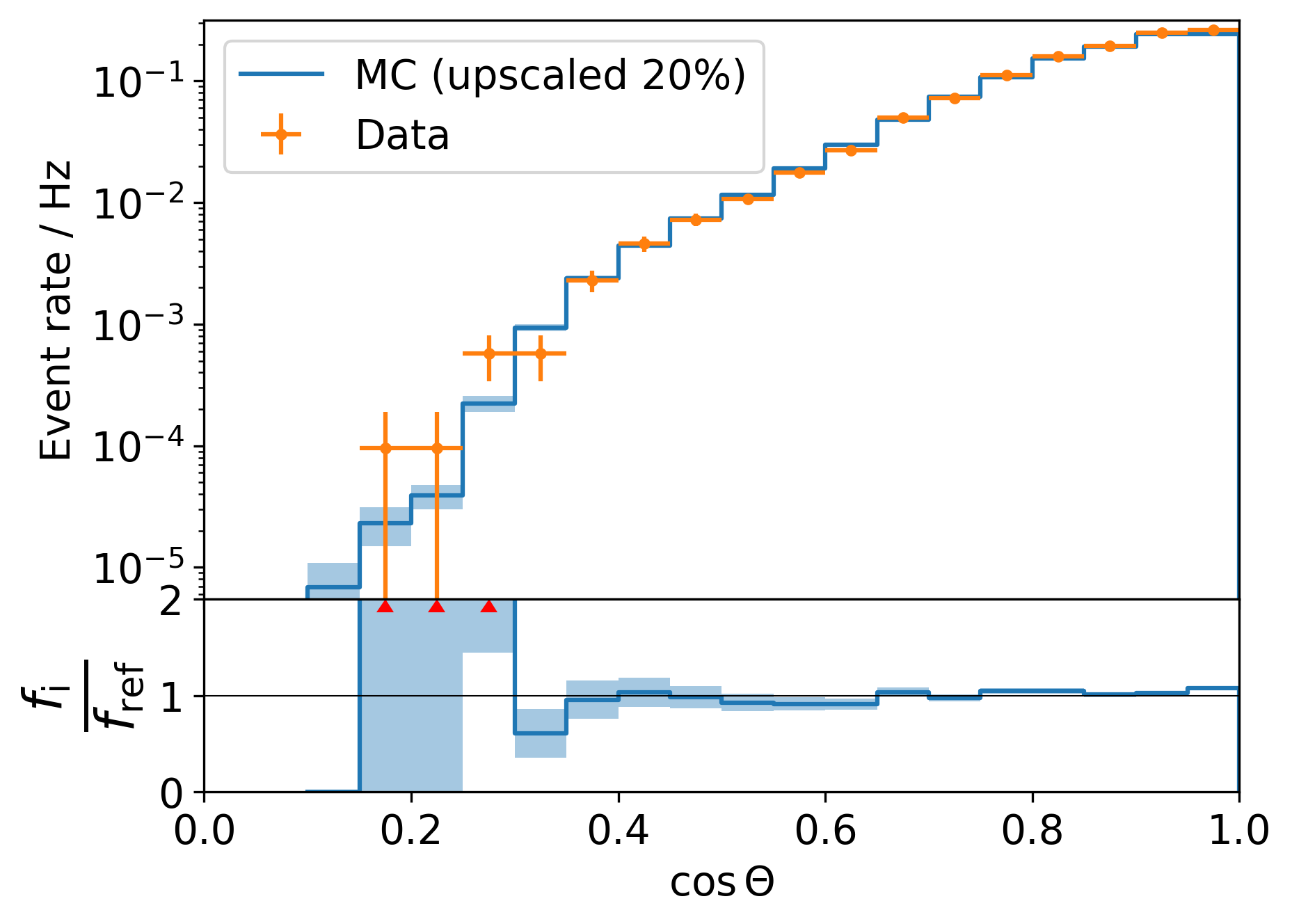
Fig. 33 : Data-MC agreement for the zenith angle with a score cut at 0.995 (top). Ratio plot Data/MC (bottom).

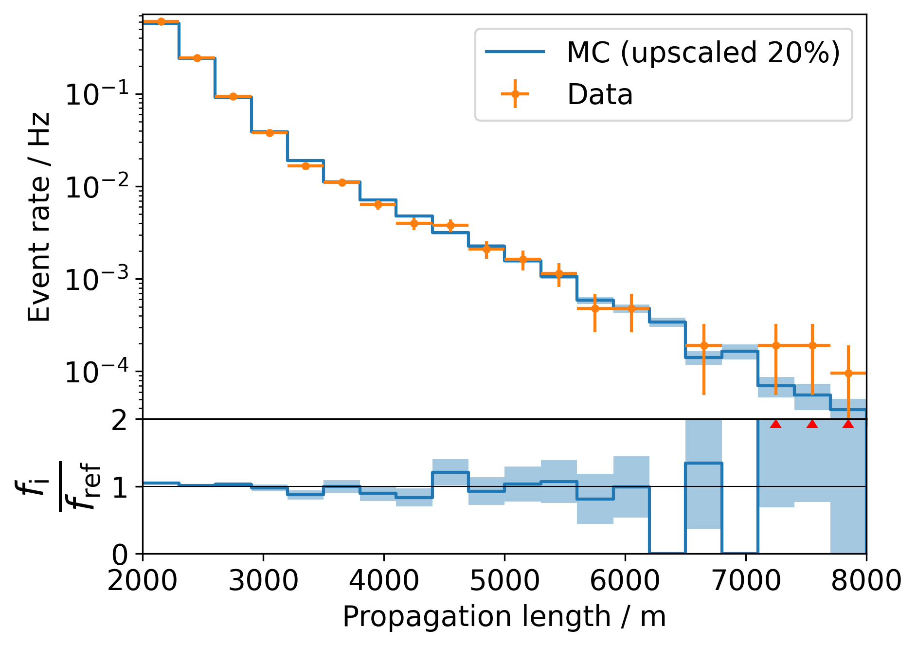
Fig. 34 : Data-MC agreement for the propagation length with a score cut at 0.995 (top). Ratio plot Data/MC (bottom).

And again in Fig. 35 - Fig. 37 with a stricter score cut at 0.999 (there is clearly a lack of statistics which makes it hard to draw any conclusions):

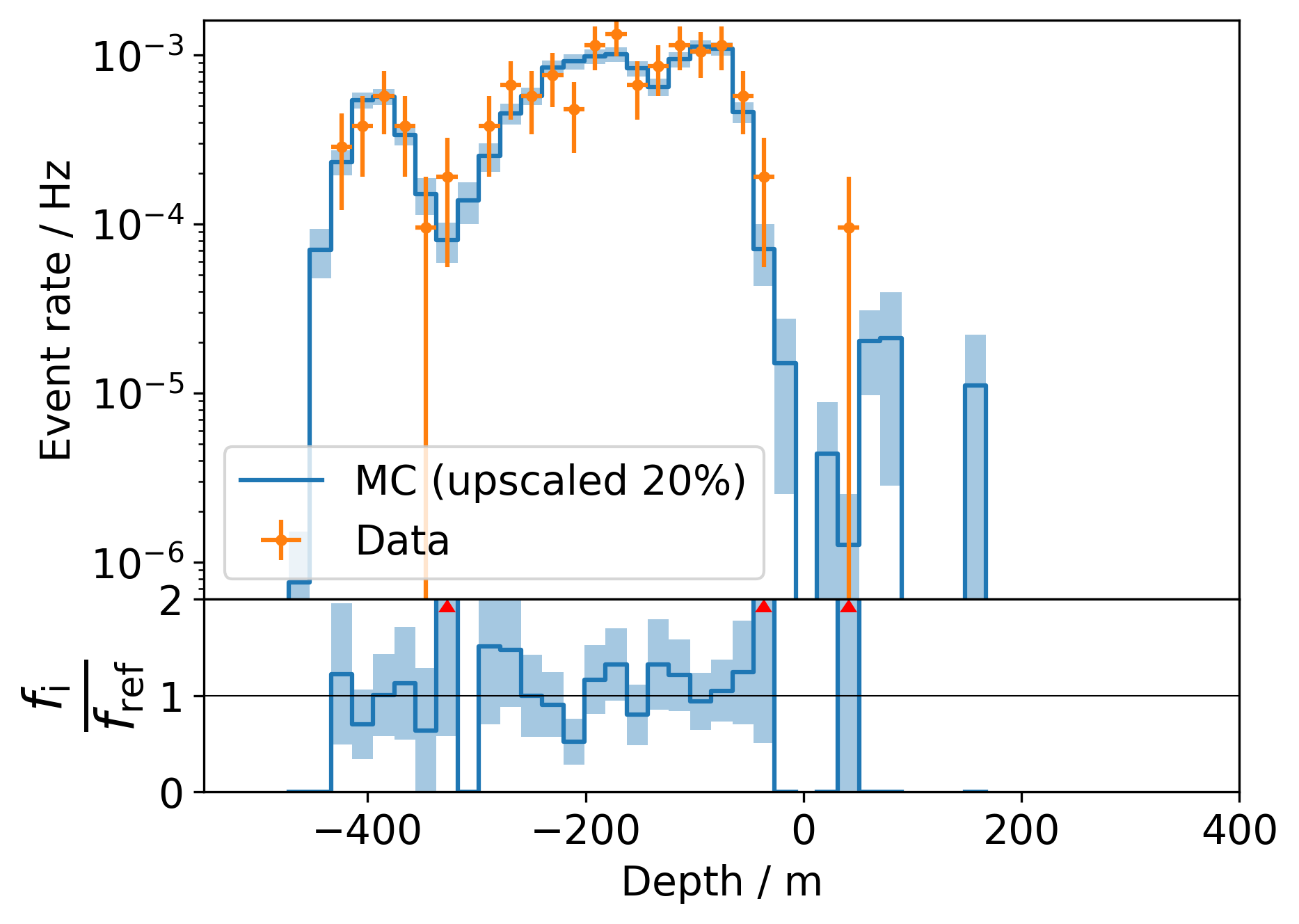
Fig. 35 : Data-MC agreement for the vertical stopping depth with a score cut at 0.999 (top). Ratio plot Data/MC (bottom).

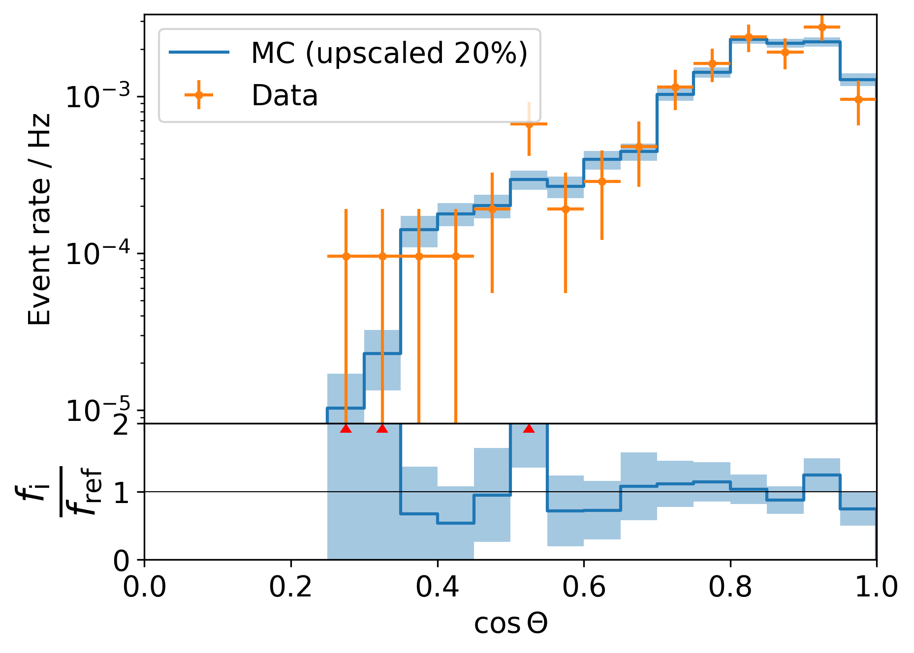
Fig. 36 : Data-MC agreement for the zenith angle with a score cut at 0.999 (top). Ratio plot Data/MC (bottom).

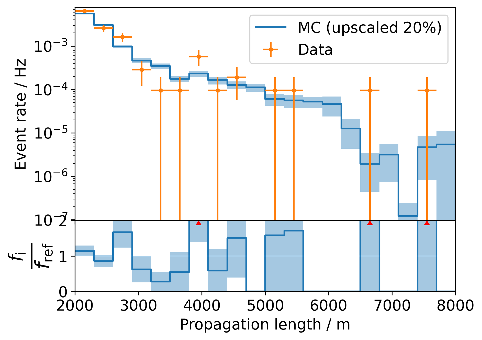
Fig. 37 : Data-MC agreement for the propagation length with a score cut at 0.999 (top). Ratio plot Data/MC (bottom).

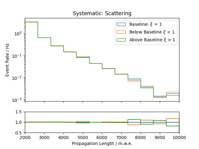
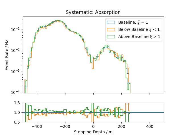
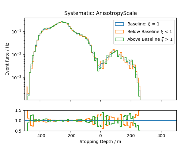
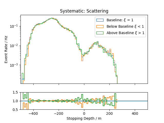
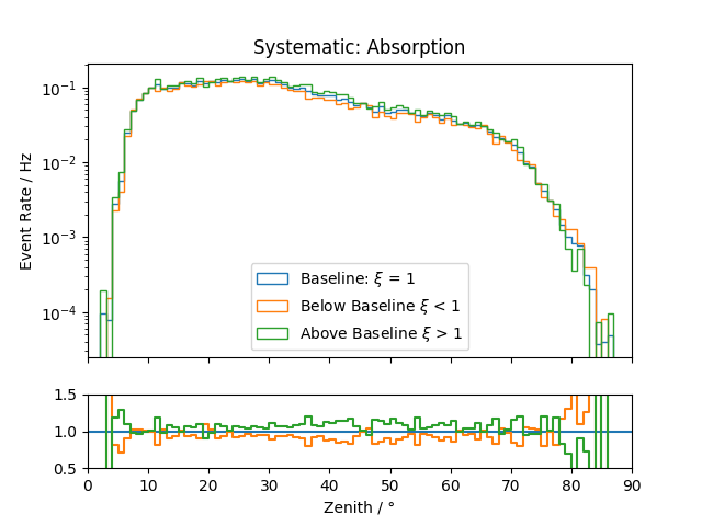
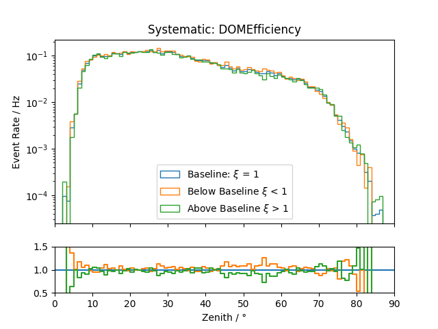
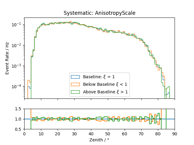
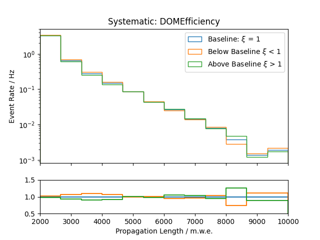
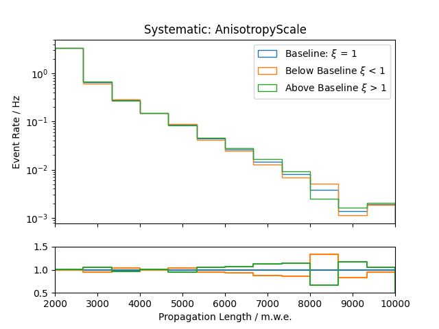
Systematic Effects

Systematic effects can also have an influence on the observable’s distributions. The distributions for all the considered systematics are shown below. They are estimated based on snowstorm simulations. The baseline distribution is the standard distribution of all events (with analysis cuts applied). Hence, the average systematic parameter amounts to the baseline value. The baseline distributions are further compared to those of events with systematic parameters below/above the baseline value, thus shifting the average parameter of the sub-set by several percent.

Stopping depth:

Zenith:

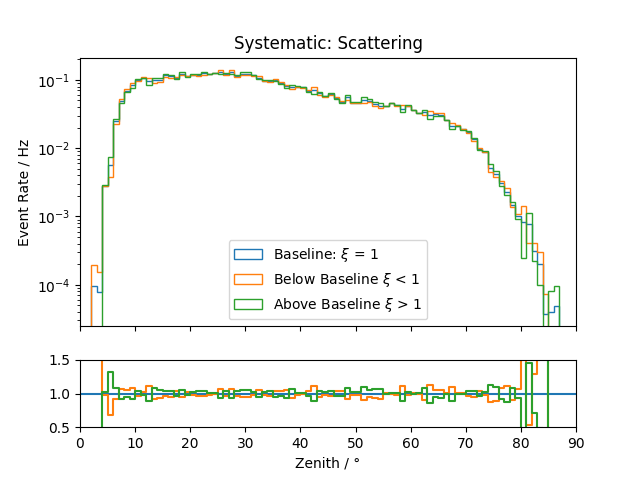
Propagation length: