Systematic Checks

Flux Models

The unfolding has to be trained on MC data which is weighted to a certain model. This could in principle have an impact on the result, although the general concept of unfolding aims to be very robust against these changes. The impact was tested by using different training models. However, the test model that the unfolding is applied to remains unchanged (GaisserH3a). The results are shown in Fig. 49 and Fig. 50. The impact of different pre-defined models appears to be small. The unfolding does not recover the MC truth perfectly, however the quality of the result does not change significantly depending on the model that is used for training.

In order to test even more extreme cases, the unfolding is performed using different offsets in the spectral index compared to the standard GaisserH3a-model. The only clear deviation arises in case of an offset of \(\Delta \gamma = 0.5\), which is considered to be quite drastic compared to the expected offsets between model and true phyisics.

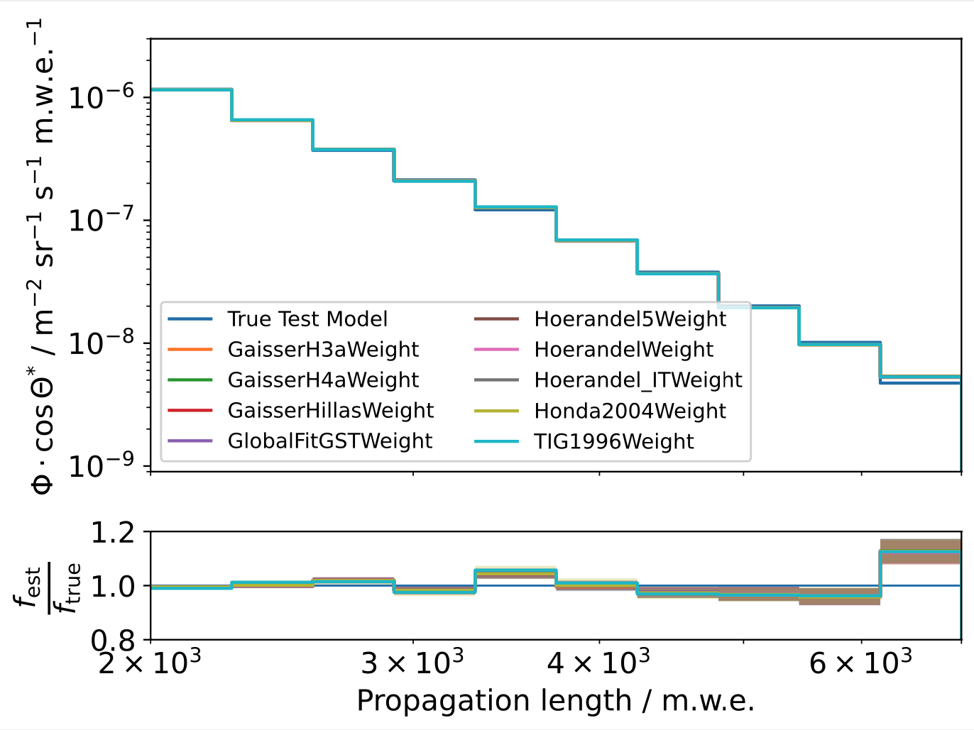
Fig. 49 : Top: Unfolding result using different pre-defined fluxmodels for training. The test model remains the same (GaisserH3a) for each iteration. Bottom: Ratio plot with the true GaisserH3a distribution as baseline.

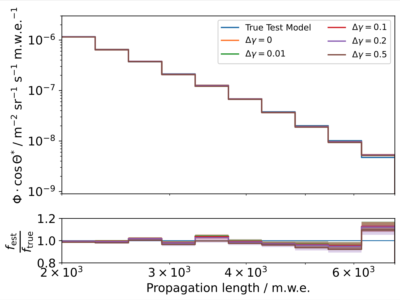
Fig. 50 : Top: Unfolding result using different deviations in the spectral index compared to the test model. The test model remains the same (GaisserH3a) for each iteration. Bottom: Ratio plot with the true GaisserH3a distribution as baseline.

Fitting Nuisance Parameters

In funfolding, systematic uncertainties are handled by fitting additional nuisance parameters to the spectrum. The change of rate in the observable bins is calculated for subsets of varying systematic parameters (using the snowstorm simulation) and then fitted with linear functions. These weighting functions are subsequently included in the detector response matrix. Thus, it is possible to find the parameters that describe the data best by including them as additional fit parameters.

Using the MCMC approach, multiple walkers explore the likelihood \(\mathcal{L}\) while moving closer to its maximum. After a series of burn-in steps they are fluctuating around the maximum, resulting in a sample of steps that resemble the a-posteriori distributions of the systematic parameters. These distributions together with the corresponding correlations are plotted below.

Fig. 51 shows the distributions of a baseline propagation length unfolding with the snowstorm set. Here, the systematic parameters of the unfolded test set are set to the baseline values, which read:

• Absorption: \(1\)

• Anisotropy: \(1\)

• DOM efficiency: \(1\)

• HoleIce (1): \(-0.025\)

• HoleIce (2): \(0\)

• Scattering: \(1\)

The distributions are very precisely centered around their expected values. It should however be noted that this test can only be performed when unfolding the first four target bins due to a lack of snowstorm statistics. For a larger range in propagation length many bins in the observable space are not populated using our self-simulated snowstorm set. Hence, this test merely serves as a proof of concept and will be repeated with the full 20904 snowstorm set on the entire length scale once the data is available.

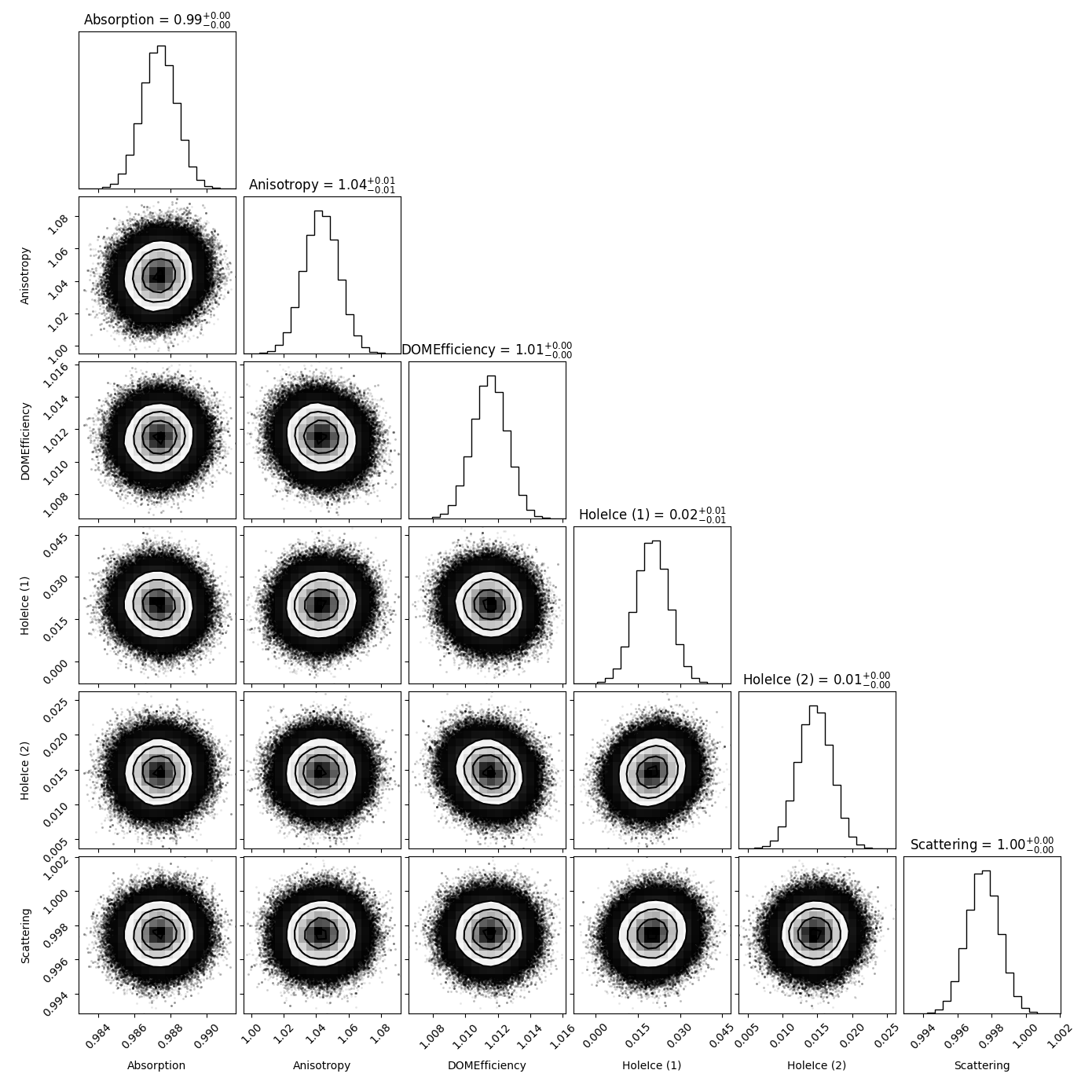
Fig. 51 : Systematic parameter correlations when unfolding the first 4 target bins in propagation length without regularization and a baseline test set.

The following plots agin show the same correlations but this time the test set consists of a snowstorm subset with one systematic parameter being varied on the order of several percent. As expected, the corresponding shifts are also visible in the resulting MCMC distributions.

In some cases there are also small shifts in parameters that are not altered in the test set (especially for the first holeice parameter). We assume these shifts to be caused by the limited statistics of the snowstrom set and the fact that we have to oversample the number of events for the unfolding to be even feasible.

Absorption:

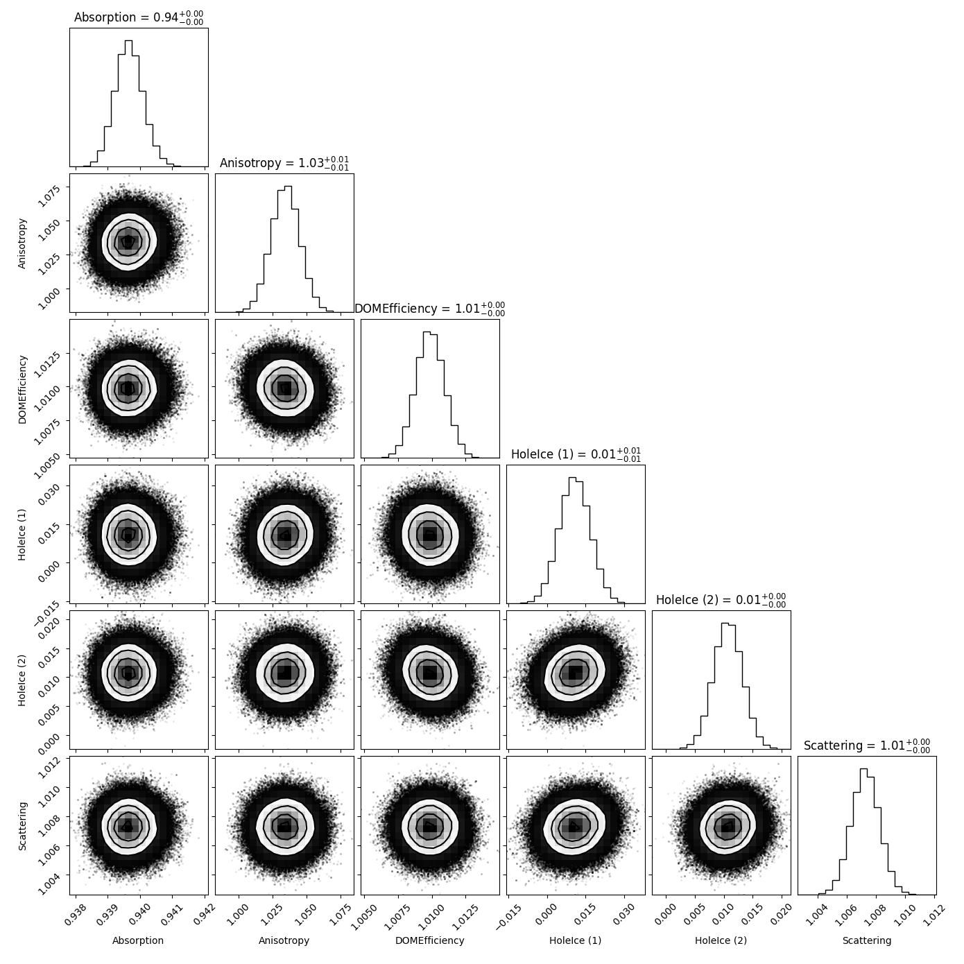
Fig. 52 : Systematic parameter correlations when unfolding the first 4 target bins in propagation length without regularization using a snowstorm test set with absorption scaled down to \(0.95\).

Fig. 53 : Systematic parameter correlations when unfolding the first 4 target bins in propagation length without regularization using a snowstorm test set with absorption scaled up to \(1.05\).

Anisotropy:

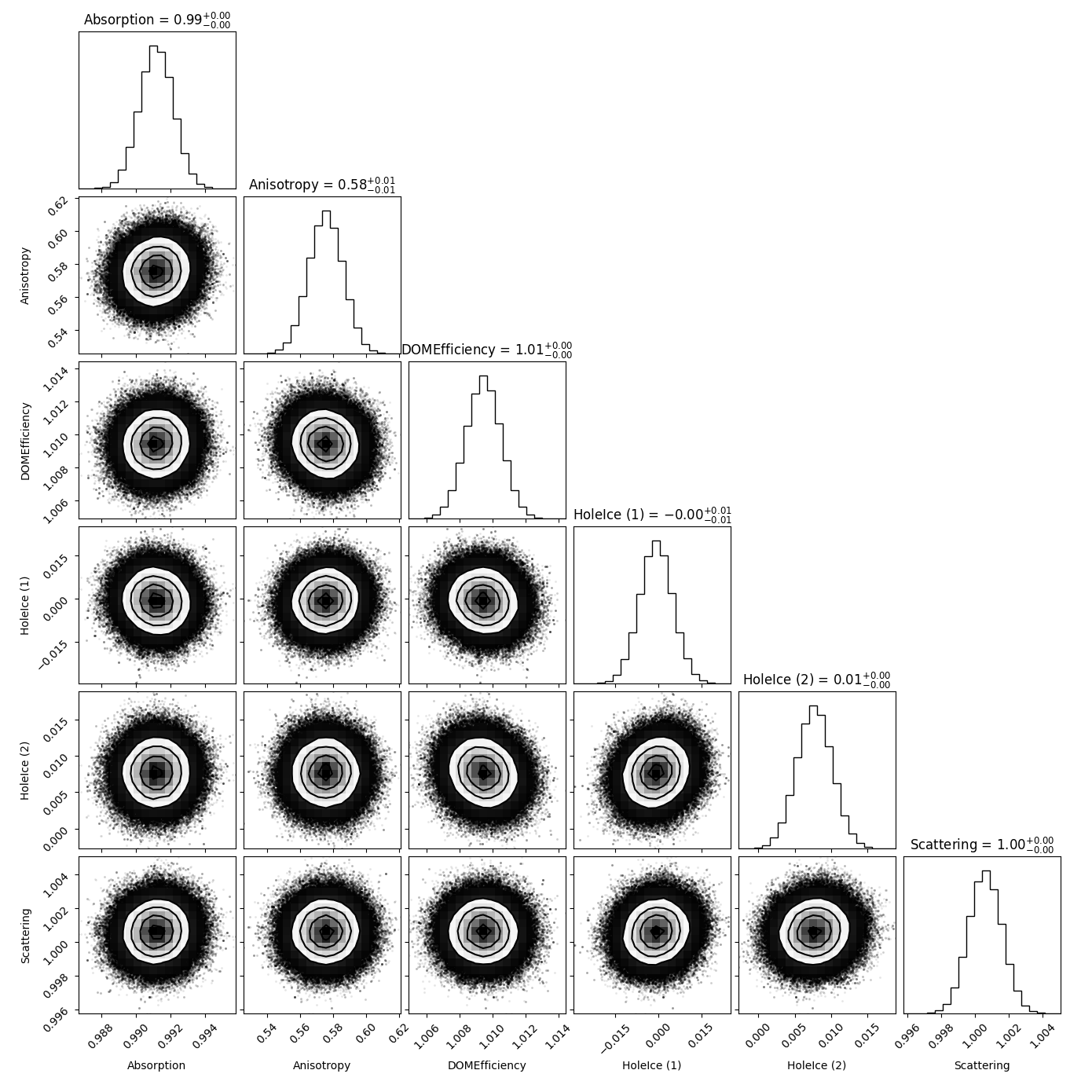
Fig. 54 : Systematic parameter correlations when unfolding the first 4 target bins in propagation length without regularization using a snowstorm test set with anisotropy scaled down to \(0.95\).

Fig. 55 : Systematic parameter correlations when unfolding the first 4 target bins in propagation length without regularization using a snowstorm test set with anisotropy scaled up to \(1.05\).

DOM efficiency:

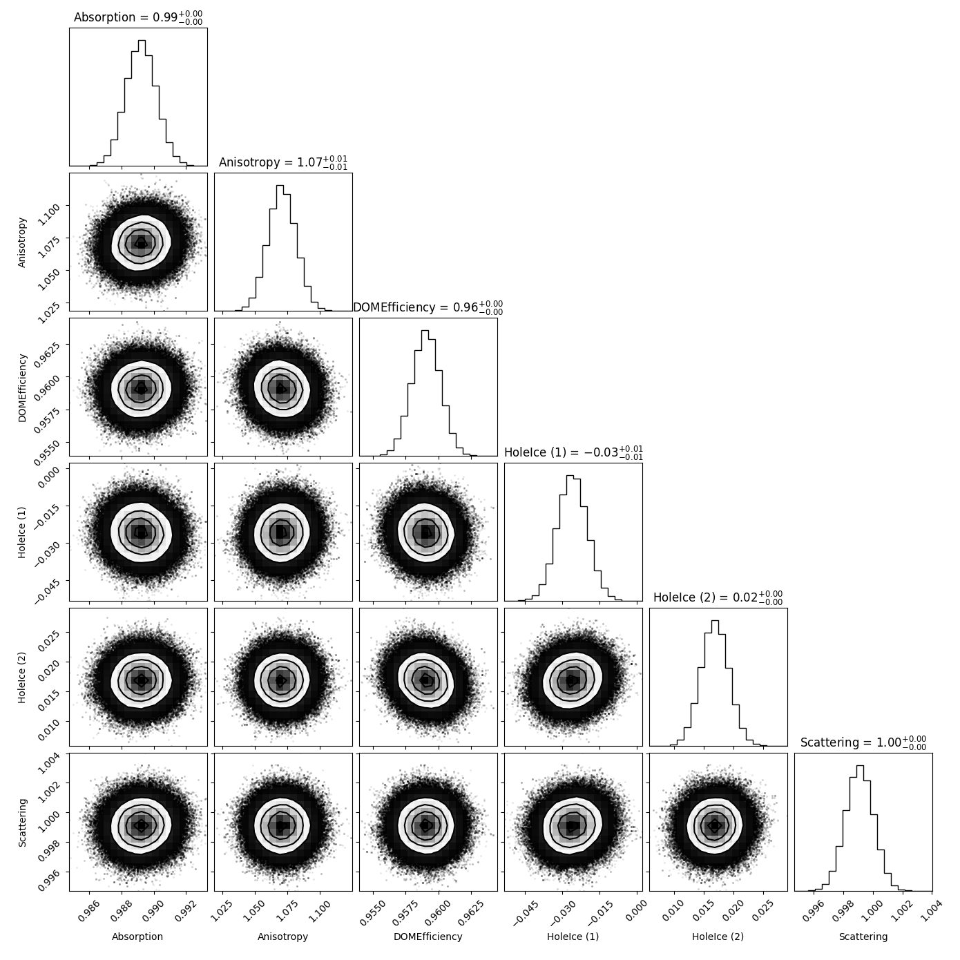
Fig. 56 : Systematic parameter correlations when unfolding the first 4 target bins in propagation length without regularization using a snowstorm test set with DOM efficiency scaled down to \(0.95\).

Fig. 57 : Systematic parameter correlations when unfolding the first 4 target bins in propagation length without regularization using a snowstorm test set with DOM efficiency scaled up to \(1.05\).

HoleIce:

Fig. 58 : Systematic parameter correlations when unfolding the first 4 target bins in propagation length without regularization using a snowstorm test set with holeice (1) scaled down to \(-0.3375\).

Fig. 59 : Systematic parameter correlations when unfolding the first 4 target bins in propagation length without regularization using a snowstorm test set with holeice (1) scaled up to \(0.2875\).

Fig. 60 : Systematic parameter correlations when unfolding the first 4 target bins in propagation length without regularization using a snowstorm test set with holice (2) scaled down to \(-0.1\).

Fig. 61 : Systematic parameter correlations when unfolding the first 4 target bins in propagation length without regularization using a snowstorm test set with holice (2) scaled up to \(0.1\).

Scattering:

Fig. 62 : Systematic parameter correlations when unfolding the first 4 target bins in propagation length without regularization using a snowstorm test set with scattering scaled down to \(0.95\).

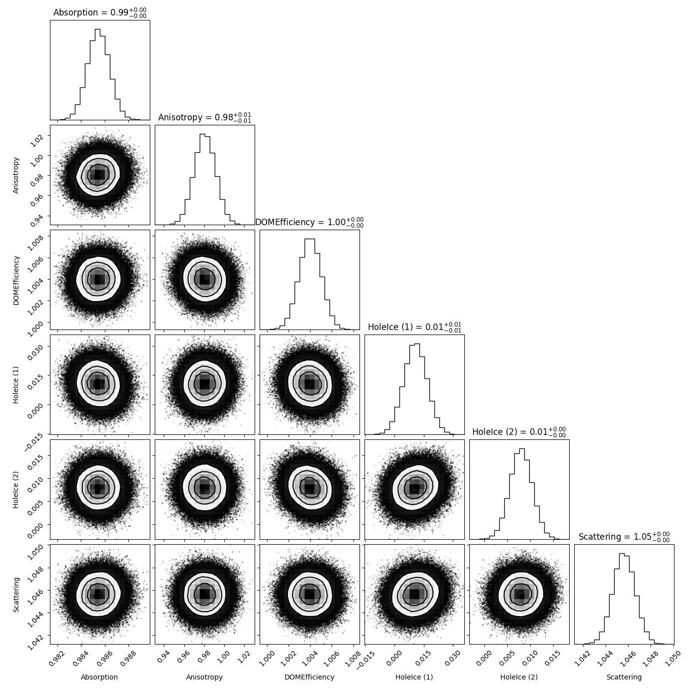
Fig. 63 : Systematic parameter correlations when unfolding the first 4 target bins in propagation length without regularization using a snowstorm test set with scattering scaled up to \(1.05\).

Impact of regularization

Regularization is an additional assumption which is integrated into the likelihood. It is designed to overcome difficulties such as ill-posed problems by introducing a penalty term that suppresses a certain behavior of the solution. This analysis uses the Tikhonov regularization, penalizing oscillations in the unfolded spectrum.

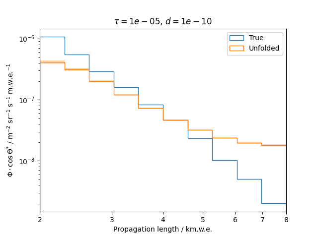
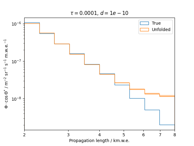
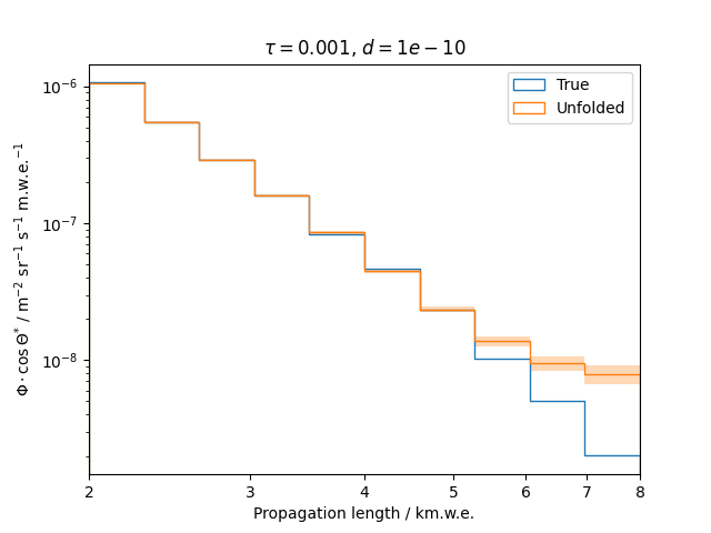
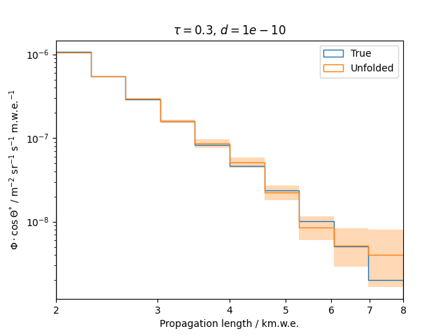
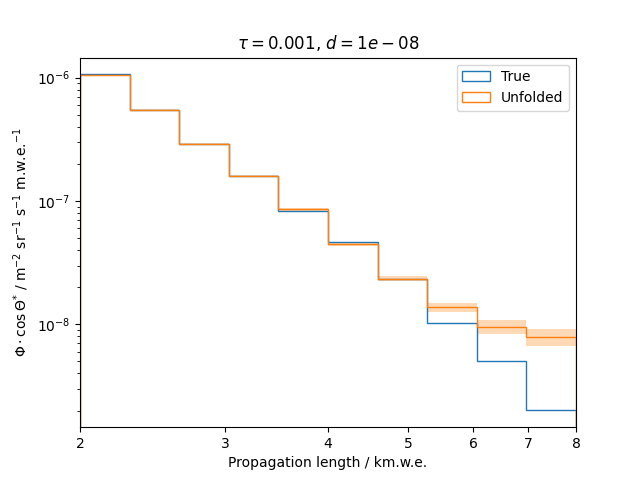
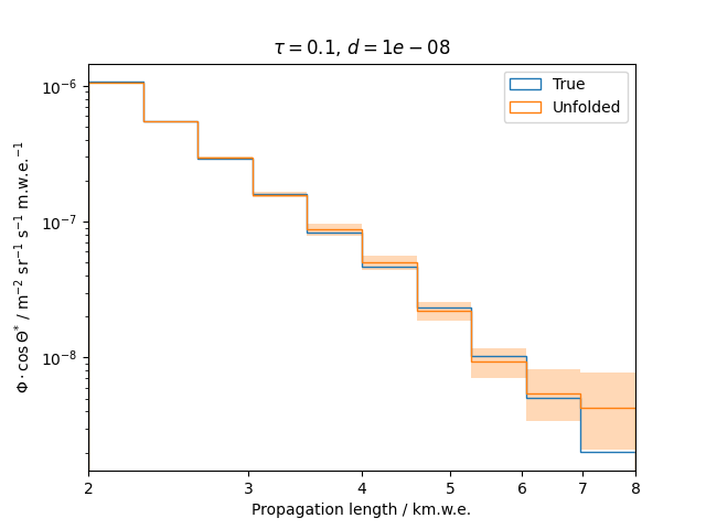
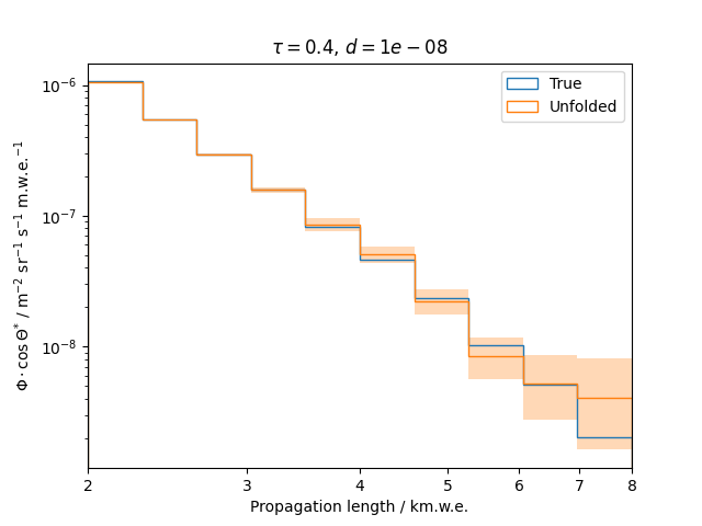
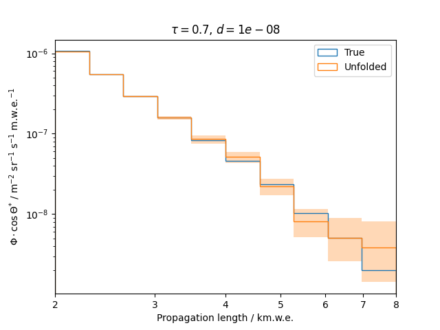
To get a feeling for how and to what extent the regularization actually impacts the unfolding, the following plots show results that were determined using various regularization strengths \(\tau\) together with different log-offsets \(d\). It is desired to use as little regularization as possible while still obtaining a comparably smooth result (the log of the specturm is expected to be flat).

\(d = 10^{-10}\) :

\(d = 10^{-8}\) :

\(d = 10^{-5}\) :

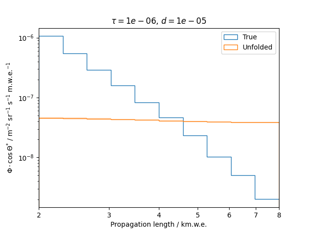
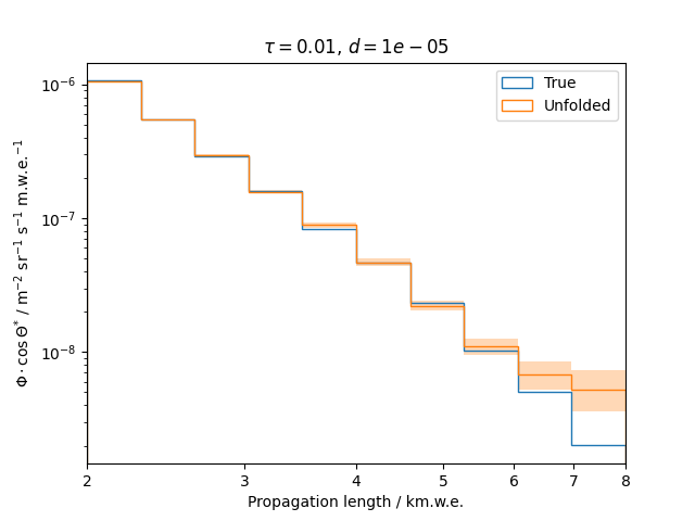
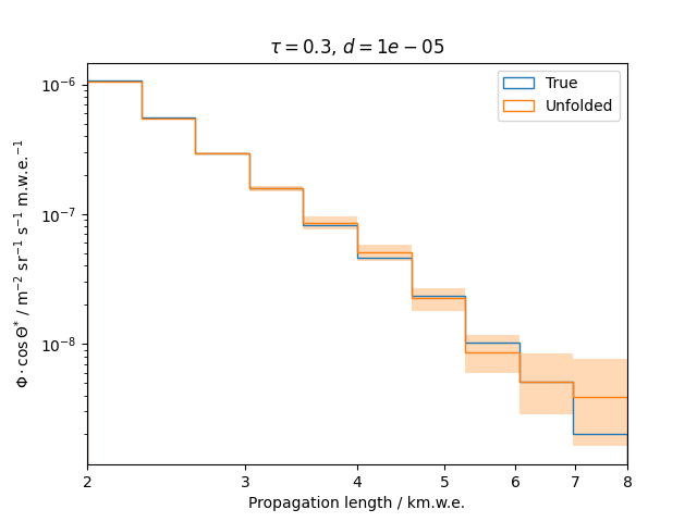
Comparing these plots shows that it is crucial to choose an appropriate regularization strength since it can drastically change the shape of the spectrum. Even with small (or even no) regularization the spectra do not seem to exhibit major oscillations due to amplified statistical noise.

The exact determination of the log-offset appears to be of minor importance since it has vanishing impact on the unfolded spectrum. It is set to a value of \(d = 1e-10\) as default in this analysis.