UNBLINDING PROPOSAL: GRB030329
ABSTRACT
The discovery of high-energy (TeV-PeV) neutrinos from gamma-ray bursts (GRBs) would shed light on their intrinsic microphysics by confirming hadronic acceleration in the relativistic jet; possibly revealing an acceleration mechanism for the highest energy cosmic rays. All AMANDA gamma-ray burst (GRB) analyses to date have featured a signal assumption based upon a diffuse ensemble of bursts described by averaged electromagnetic parameters. We describe novel modeling techniques used in an analysis featuring three models based upon confronting the fireball phenomenology with ground-based and satellite observations of GRB030329, which triggered the High Energy Transient Explorer (HETE-II). Contrary to previous diffuse searches, the expected discrete muon neutrino energy spectra for models 1 and 2, based upon an isotropic and beamed emission geometry, respectively, are directly derived from the fireball description of the prompt g-ray photon energy spectrum, whose spectral fit parameters are characterized by the Band function, and the spectroscopically observed redshift, based upon the associated optical transient (OT) afterglow. For comparison, we also consider a model (3) based upon averaged burst parameters. Strict spatial and temporal constraints (based upon electromagnetic observations), in conjunction with a single, robust cut on maximum search bin radius (Ψma x≤ ~20 degrees), have been leveraged to realize a nearly background-free search (rejecting ~99% of the background while retaining ~86% of the signal for all three models), using 2003 level 2 filtering data from the Zeuthen multi-year AMANDA-II data set. Our preliminary results yield a peak neutrino effective area of ~100 m2 at ~2 PeV and a sensitivity of ~1.46x10⁻¹ GeV/(cm2 s) for model 1. Using the same theoretical framework, the detector response of AMANDA-II and IceCube to spectra based upon discrete and averaged parameters are discrepant in mean neutrino energy and event rate by over an order of magnitude. Such variance in the detector response, which directly translates into observables such as expected number of neutrino events, unequivocally demonstrates the value of a discrete modeling approach when making correlative neutrino observations of individual bursts. Based upon our preliminary analysis described above, we formally request approval for the unblinding of GRB030329.
The 2005 ICRC Proceedings serves as an executive summary of this analysis.
1. Introduction
2. Electromagnetic Parameters
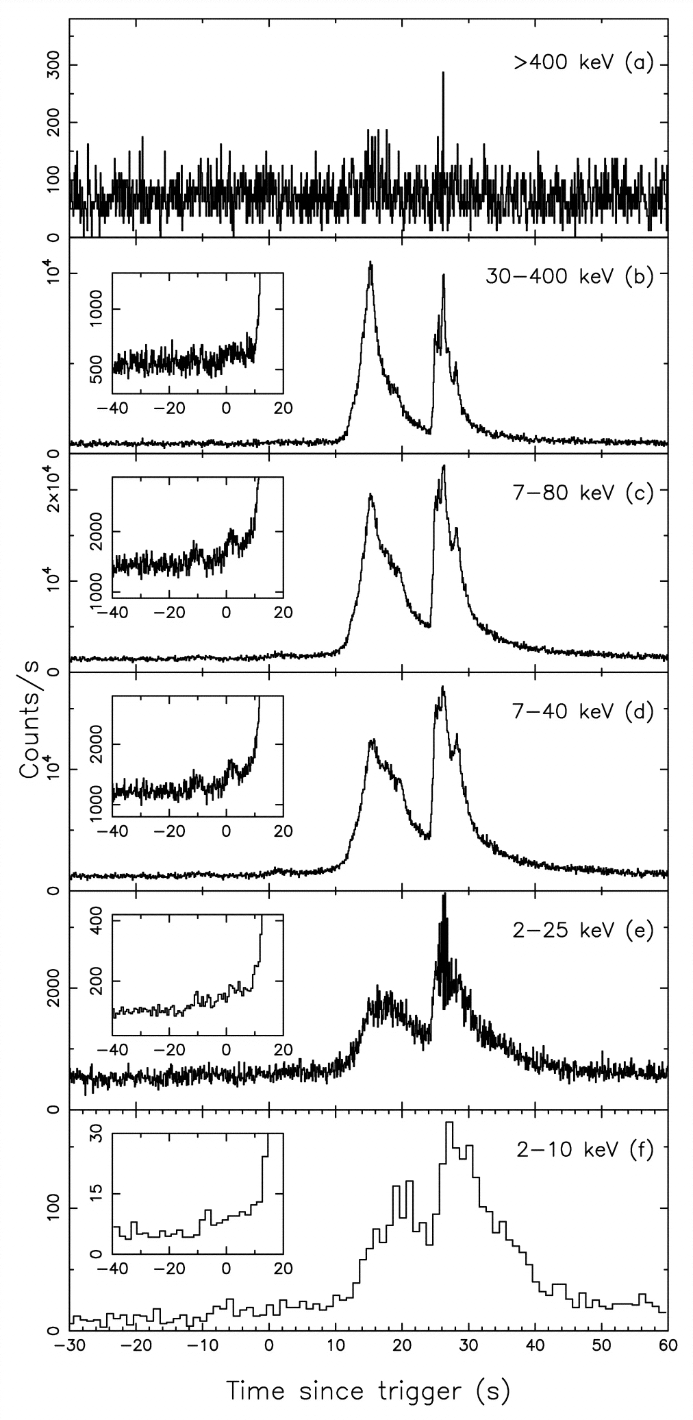
On March 29, 2003 @ 11h37m14.s67 (UTC), HETE-II was triggered by GRB030329, resulting in the following light curve (temporal spectrum):
Due to the rapid communication between ground-based and satellite detectors provided by the GCN, electromagnetic observation of the prompt g-ray and multi-afterglow emission revealed the following observables:
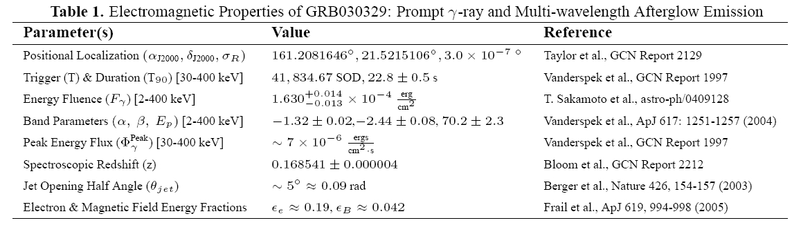
Based upon the above, we found that the photon break energy was egb ~116 keV, the isotropic peak luminosity is Lgiso ~ 5.24 x 1050 ergs/s and the beamed corrected luminosity is Lgjet ~ 1.99 x 1048 ergs/s. It should be pointed out that GRB030329 was a watershed transient, confirming the GRB-Supernova connection and revealing the in viability of the cannonball model and support for the fireball description.
3. Constructing the Neutrino Spectrum
Leptons in coincidence with the prompt g-ray emission arise via photomeson interactions:
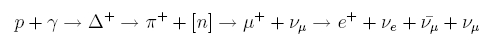
Since the ambient prompt g-rays function as the target field, subsequent neutrino emission traces the photon spectrum, which is described by the Band function:
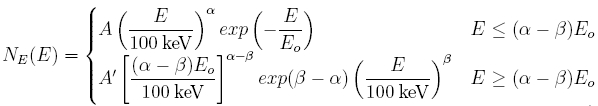
where (a-b)Eo ≡ egb. The expected neutrino energy spectrum may then be parameterized via:
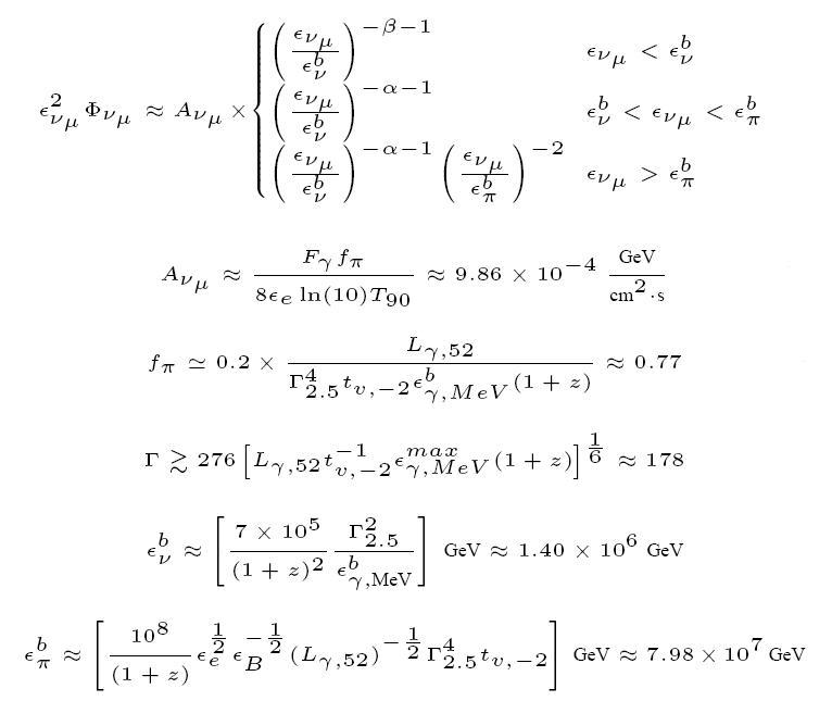
Where Lg ≡ Lg,52 (1052 ergs/s), G ≡ G2.5 (102.5), tv ≡ tv,-2(10 ms), egb ≡ ebg,MeV (1 MeV), eg ≡ emaxg,MeV (100 MeV). Three models were generated using the following parameters:
| Parameter | Discrete Isotropic Emission (Model 1) | Discrete Jet Emission (Model 2) | Average Isotropic Emission (Model 3) |
| Photon energy fluence, Fg (ergs/cm2) | 1.63E-4 | 1.63E-4 | 6E-6 |
| redshift, z | 0.168541 | 0.168541 | 1 |
| Luminosity, Lg (ergs/s) | 5.24E50 | 1.99E48 | 1E52 |
| Bulk Lorentz Boost Factor, G | 178 | 70 | 300 |
| Proton Efficiency, fp | 0.77 | 0.12 | 0.2 |
| Neutrino Flux Normalization, Anm | 9.86E-4 | 1.54E-4 | 8.93E-6 |
| Neutrino break energy, enb (GeV) | 1404951 | 219343 | 1E5 |
| Pion Synchrotron break energy, epb (GeV) | 79832941 | 31543774 | 1E7 |
| Low energy photon spectral index, a | -1.32 | -1.32 | -1 |
| High energy photon spectral index, b | -2.44 | -2.44 | -2 |
The neutrino spectral models and the response of AMANDA-II and IceCube are illustrated below:
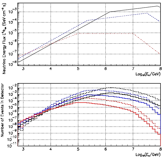
Upper panel - Prompt neutrino energy flux for models 1 (solid black), 2 (dashed blue) and 3 (dot-dashed red), based upon the above parameterization. Lower panel - Detector response for models 1 (black), 2 (blue) and 3 (red) for AMANDA-II (sold) and IceCube (dashed). The effects of neutrino flavor oscillations have been included.
| Model | Number of Signal Events in AMANDA (nsA) | Number of Signal Events in IceCube (nsI) |
| 1. GRB030329 Isotropic Emission | 2.0E-2 | 1.3E-1 |
| 2. GRB030329 Jet Emission | 1.2E-2 | 6.9E-2 |
| 3. "Average" burst | 7.6E-4 | 3.8E-3 |
The values in the above table are based upon a 40 second emission, before cuts. One immediately notices that the peak of the energy response distribution in both AMANDA-II and IceCube is coupled to the first break energy of the spectrum, i.e. egb, which is based upon observables such as the spectroscopic redshift and photon break energy (gleaned from the Band spectral fit parameters). Clearly, the response of the detector varies due to the input signal spectrum. The specific case of the three models tested in this analysis, the variance was over an order of magnitude in both mean neutrino energy and event rate. Since this directly translates into the number of expected neutrino events on-time, it effects the sensitivity and the astrophysical interpretation of a null detection. Hence, this is an unequivocal demonstration of the value in using spectra which are constructed from the electromagnetic observables associated with the bursts we observe.
4. Extraction Intervals, Detector Stability & Background Event Rate
This analysis is based upon 2003 level 2 filtering data from the Zeuthen multi-year AMANDA-II data set (at the Berkeley meeting we presented investigations at level 4).
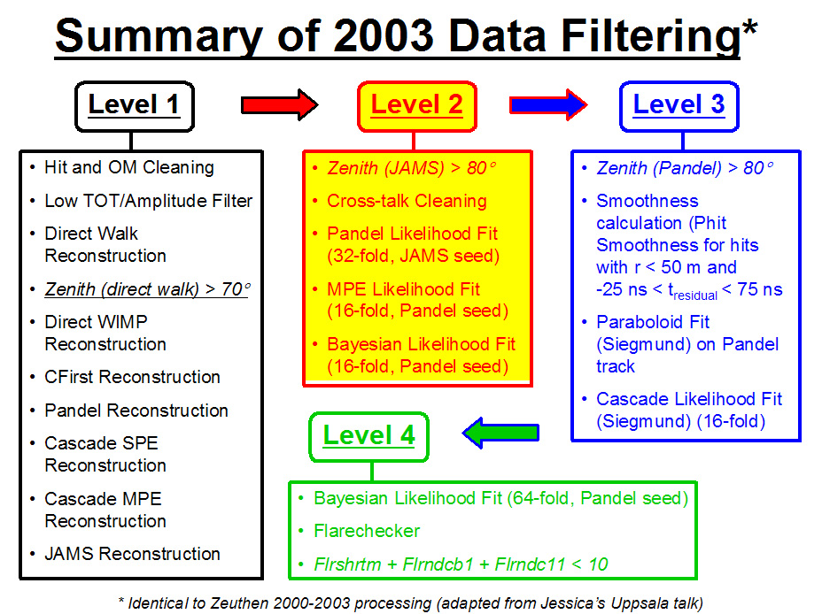
Details regarding data processing and filtering may be found here, while details regarding the simulation files may be found here. Traditionally, a 2 hour interval, centered upon the burst trigger time, has been used to characterize the background and determine detector stability in AMANDA GRB analyses. For this analysis, we explored multiple extraction intervals from 2 to 20 hours, which spanned runs 7001-7002. A regiment of diagnostic plots which include the number of events in a 10 second interval, the time between consecutive events and GMTSEC may be found here. The distribution of the number of events in a 10 second interval was consistent with a Gaussian fit for all extracted intervals. Details regarding investigations of cross-talk and flare checking my be found elsewhere.
The best characterization of background was achieved with the 20 hour extraction interval. However, only small fluctuations in background and detector dead-time (due to the VLF veto and DAQ buffer) were observed among the other various extraction intervals, as can be seen from the plots below:
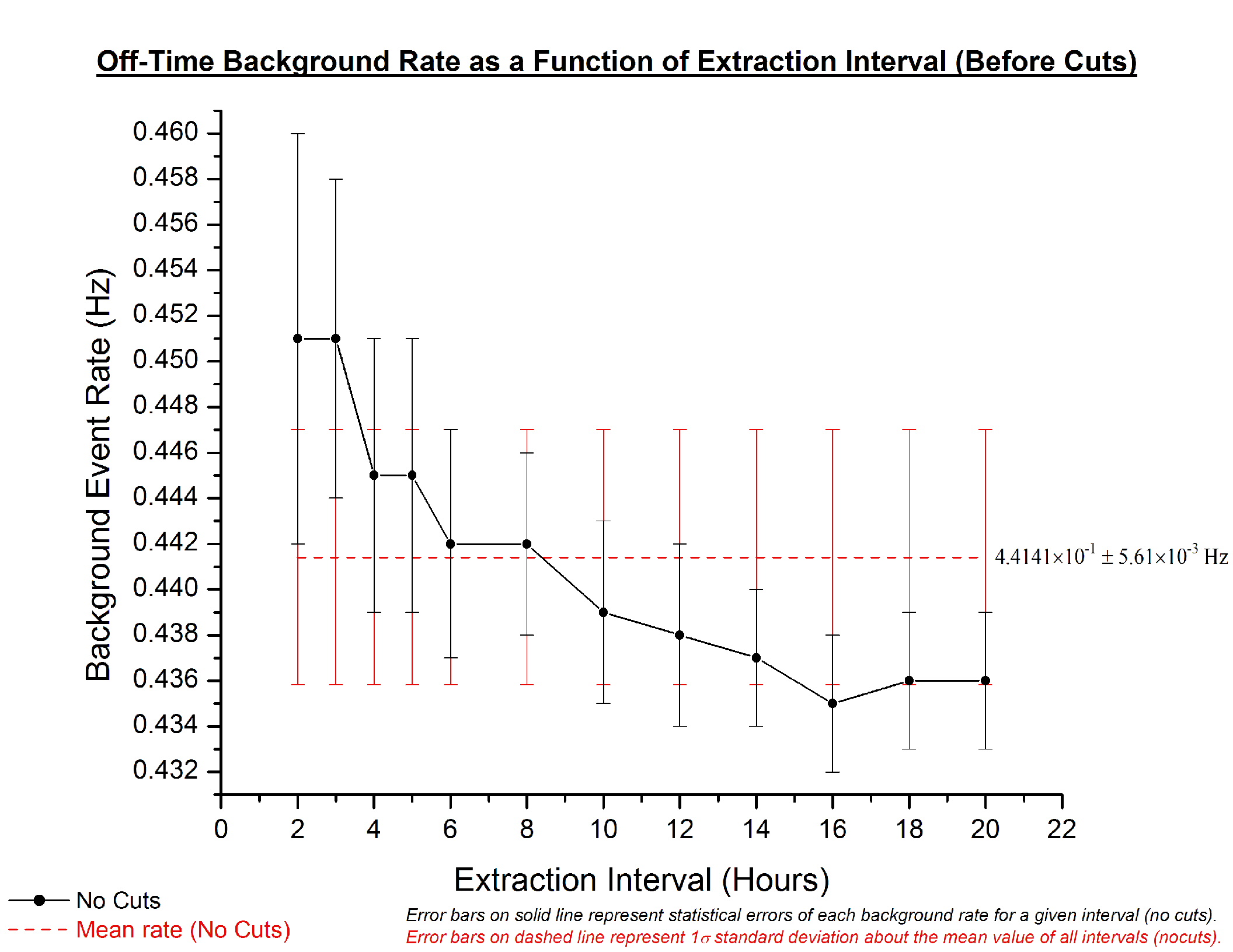
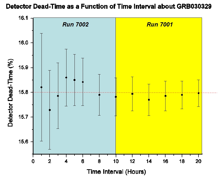
The 20 hour (72,000 second) extraction, centered on the burst trigger time spanned runs 7001-7002. A 10 minute blinded, also centered on the trigger time was invoked in order to facilitate an unbiased analysis, as illustrated below for a generic (2xh) extraction interval:
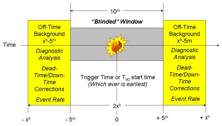
The total off-time background interval was corrected for (i) the 10 minute blinded window, (ii) detector down-time (between runs 7001 and 7002) and (c) detector dead time, amounting to a total of 57328.04 seconds, over which a total of 24,972 +/- 158 events accrued. More details regarding our assessment of the total off-time interval may be found here. Hence, the background event rate was 0.436 +/- 0.003 Hz. Based upon a visual inspection of the light curve and personal communications with members of the HETE-II collaboration, it was decided that a 40 seconds search window, taken with respect to the trigger time, would be used. This translates to an expectation of ~17.44 background events in AMANDA-II (nbA) on-time before cuts.
5. Cut Optimization: The Robustness of the Search Bin Radius
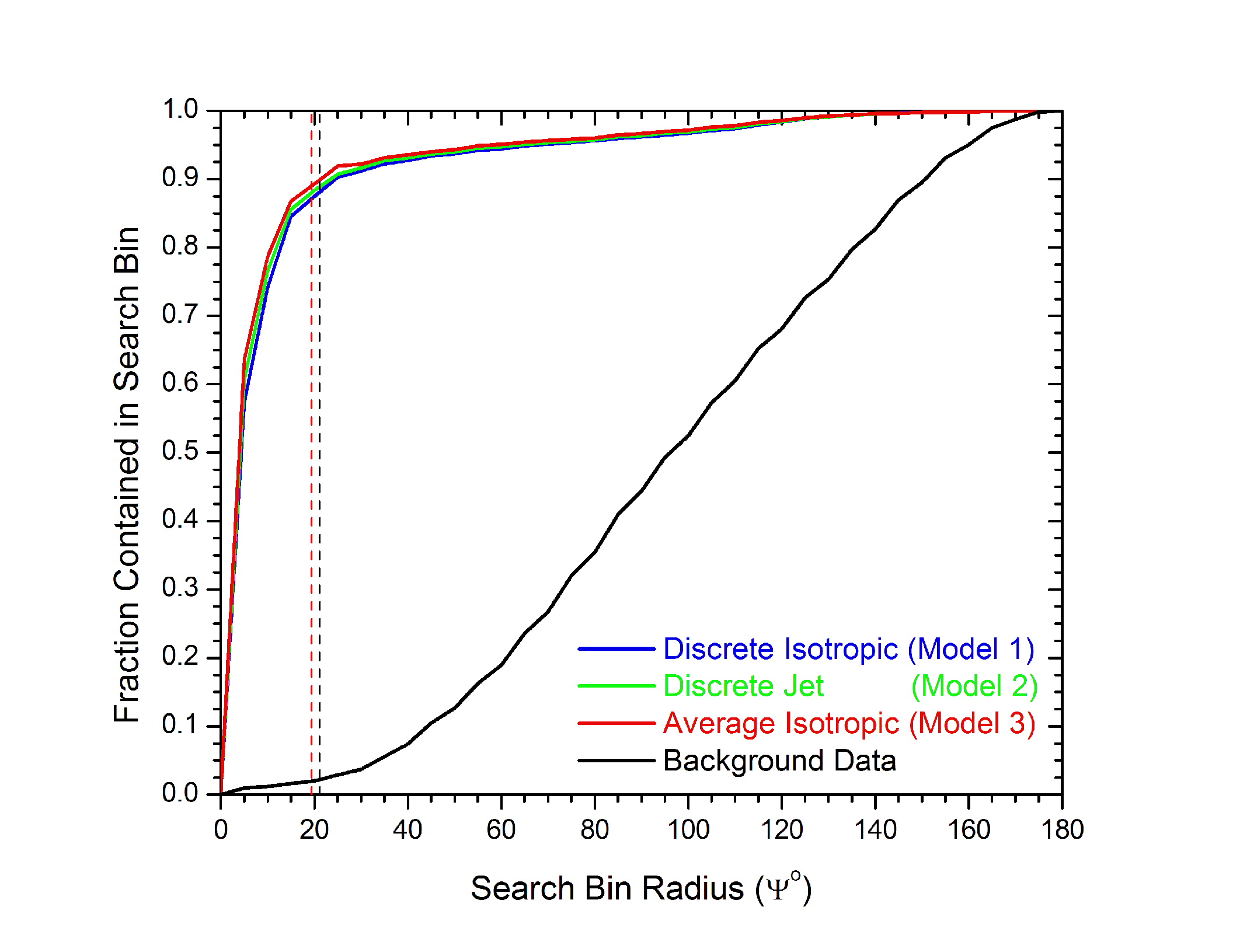
Traditionally, multiple observables have been used to optimize the cut selection in GRB analyses. Using this as a guide, we began investigating canonical observables such as nch, ndirc and search bin radius (see distributions). A modified version of the optimization algorithm used in the point source analysis was utilized in this analysis (details may be found here). The results of the optimization, i.e. minimization of the MRF, revealed that only a single, robust cut on the maximum search bin radius [Ymax (degrees) ≡ the space angle between the reconstructed muon trajectory and the positional localization vector of the GRB, defined by the radio afterglow] was required to eliminate ~99% of the background while retaining ~86% of the signal for all models. The relevant optimization plots may be found here. Below, we include plots which establish the value and efficiency of Y for each model, summarized in the table below:
|
|
Maximum Search | AMANDA-II | IceCube |
|
AMANDA-II | |||
| Model (Fn) | Bin Radius | Number of Background Events | Number of Signal Events | Number of Signal Events | MRF | Sensitivity | ||
|
|
Ymax (degrees) | Before Cuts | After Cuts | Before Cuts | After Cuts | No Cuts | GeV/(cm2 s) | |
| 1, Isotropic | 21.2 | 17.4 | 0.17 | 2E-2 | 1.7E-2 | 1.3E-1 | 148 | 1.46E-1 |
| 2. Jet | 21.2 | 17.4 | 0.17 | 1.2E-2 | 1E-2 | 6.9E-2 | 255 | 3.93E-2 |
| 3. Average isotorpic | 19.4 | 17.4 | 0.14 | 7.6E-4 | 6.5E-4 | 3.8E-3 | 3915 | 3.5E-2 |
For completeness we also include nch distributions as well as tbox plots of nch vs. Y:
Top Panel - On-time background nch distribution for background before cuts (black ~ 17.4 events) and after cuts for models 1, 2 and 3 (blue ~0.17, green ~0.17 and red ~0.14, respectively .). Bottom panel - On-time signal channel distribution for models 1, 2 and 3 (same color scheme as upper panel) for before (solid) and after (dashed) cuts.


A summary of the relevant plots for sections 4 & 5 may be found here.
6. Effective Areas
The effective neutrino and muon areas are illustrated below.
Color scheme: Optimized AMANDA-II areas for models 1 (dashed black), 2 (dashed blue) and 3 (dot-dashed red) and predicted IceCube (solid black) curves illustrated for a declination of ~22 degrees (J2000).
7. Optimization Revisited: Discovery Potential vs. Upper Limit Sensitivity
Olga has raised the following point:
"The analysis has been optimized for
limit setting as far as I understand. It seems to me that given a
specific well described burst the optimization
should be for detection. Gary is an expert on this ... but the
unblinding should be done in such a way as not to preclude optimization
for detection."
This particular point really
addresses a much larger issue of how (all) analyses are optimized in
AMANDA. Following canonical procedures, we have optimization the cuts
for the best average upper limit (sensitivity) set at the 90% C.L.
using the standard Model Rejection Potential technique, as described above. In order to
ascertain how the optimization is effected by a "discovery" or
"detection" approach, I utilized a method, developed by Gary and used
in Jessica's Diffuse analysis, which is based upon a reverse
engineering approach. This deserves a more formal introduction by Gary,
but, in short, one defines the criterion for discovery, i.e. number of
observed events at a certain confidence interval and statistical power.
One can then construct an average minimum flux that is required to
satisfy the discovery criterion, which, similar to the construction of the MRF, can
be optimized via global minimization. For lack of any nomenclature, I initially called
this minimum average flux factor the "Discovery Flux Factor" (DFF), however, we
have since changed this to the "Model Discovery Factor" (MDF) in keeping with
the analogy to the "Model Rejection Factor" (MRF).
It is instructive to first look at a naive optimization based upon minimizing the ratio of the square root of the background to the signal:
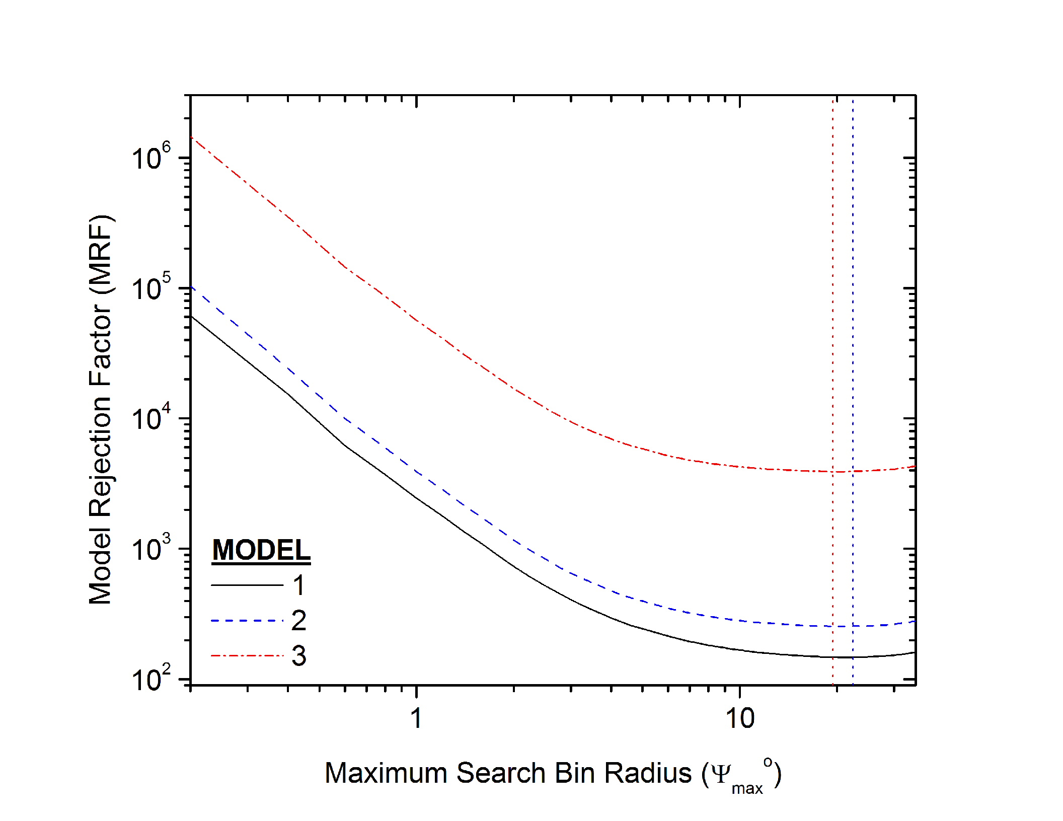
However, the above is only appropriate for in the Gaussian limit and we are in the Poissonian regime. The canonical approach used for optimizing our limit setting potential is the familiar Model Rejection Potential (MRP) method. The MRF as function of search bin radius is a continuous function, plotted for all three models at different confidence intervals below:
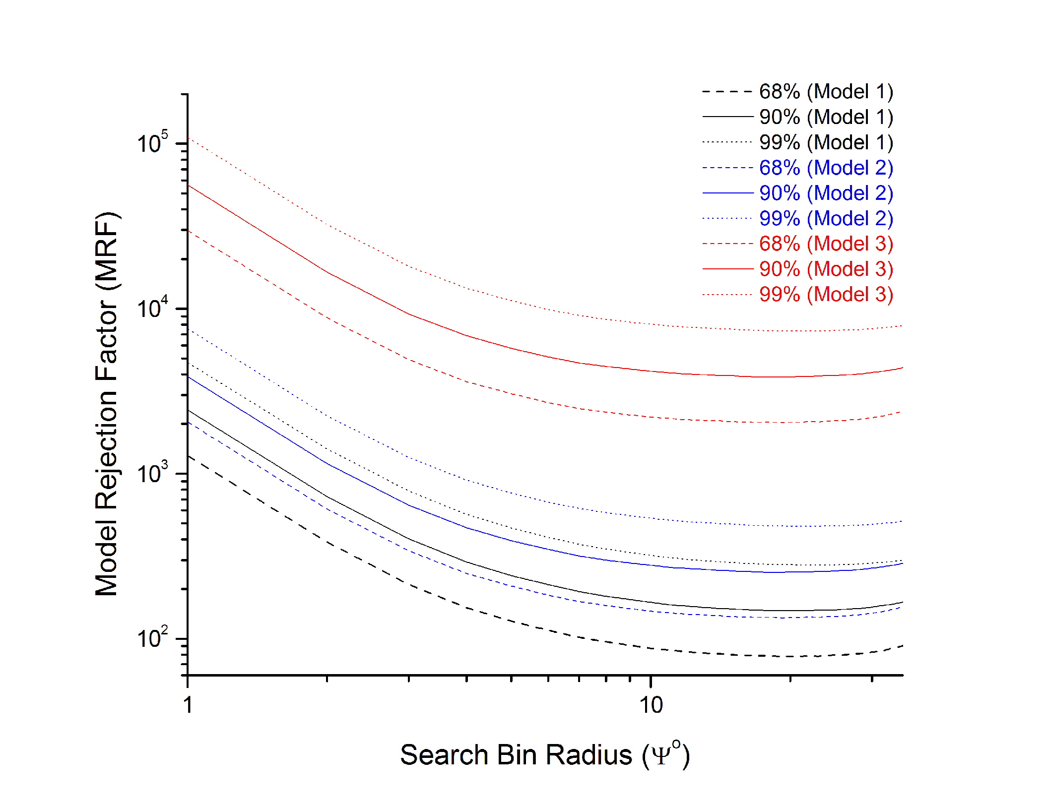
As previously stated, if one is interested in the discovery potential, then the "Model Discovery Potential" (MDP) may be used. In the plots below, I have superimposed, for each model (1-3), the various possible minimization curves. In particular, the MDF is given for 6 different levels of discovery (1-5 sigma and 90%). The discontinuity observed in the MDF curves is a consequence of the discrete nature of the Poissonian statistics used. As you increase the search bin radius, more background is accumulated and hence the number of events required to satisfy the discovery criterion increases Each successive event increase, causes a discontinuous jump in the MDF curve.
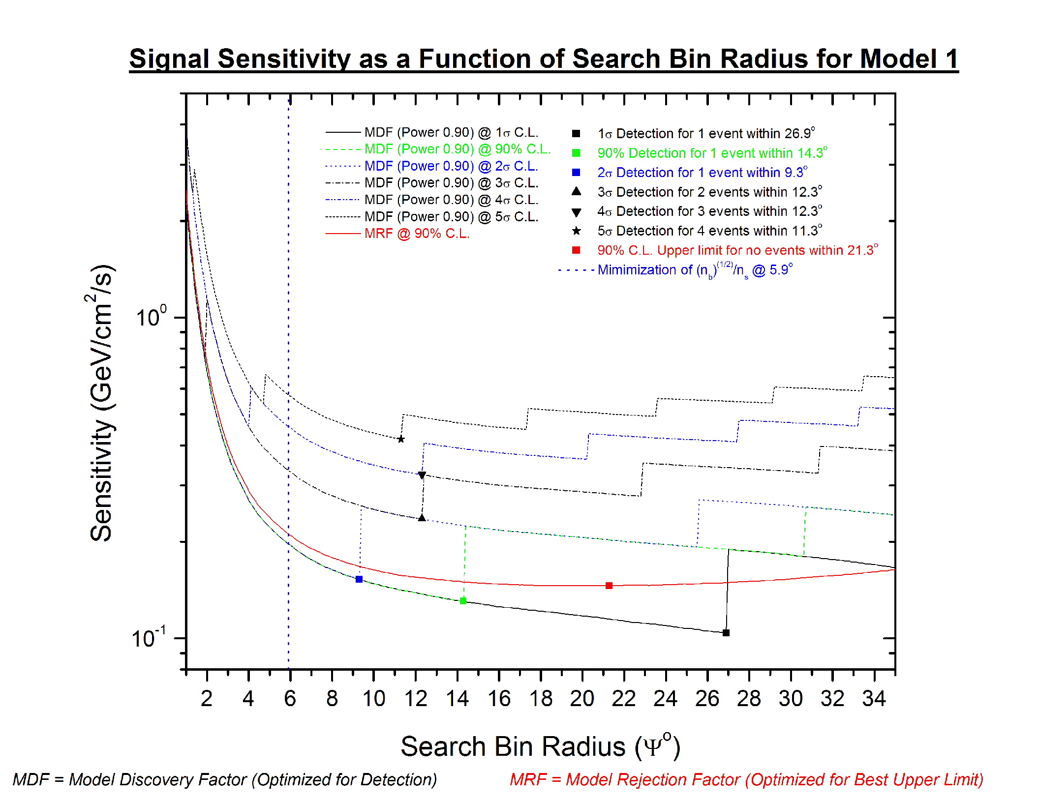
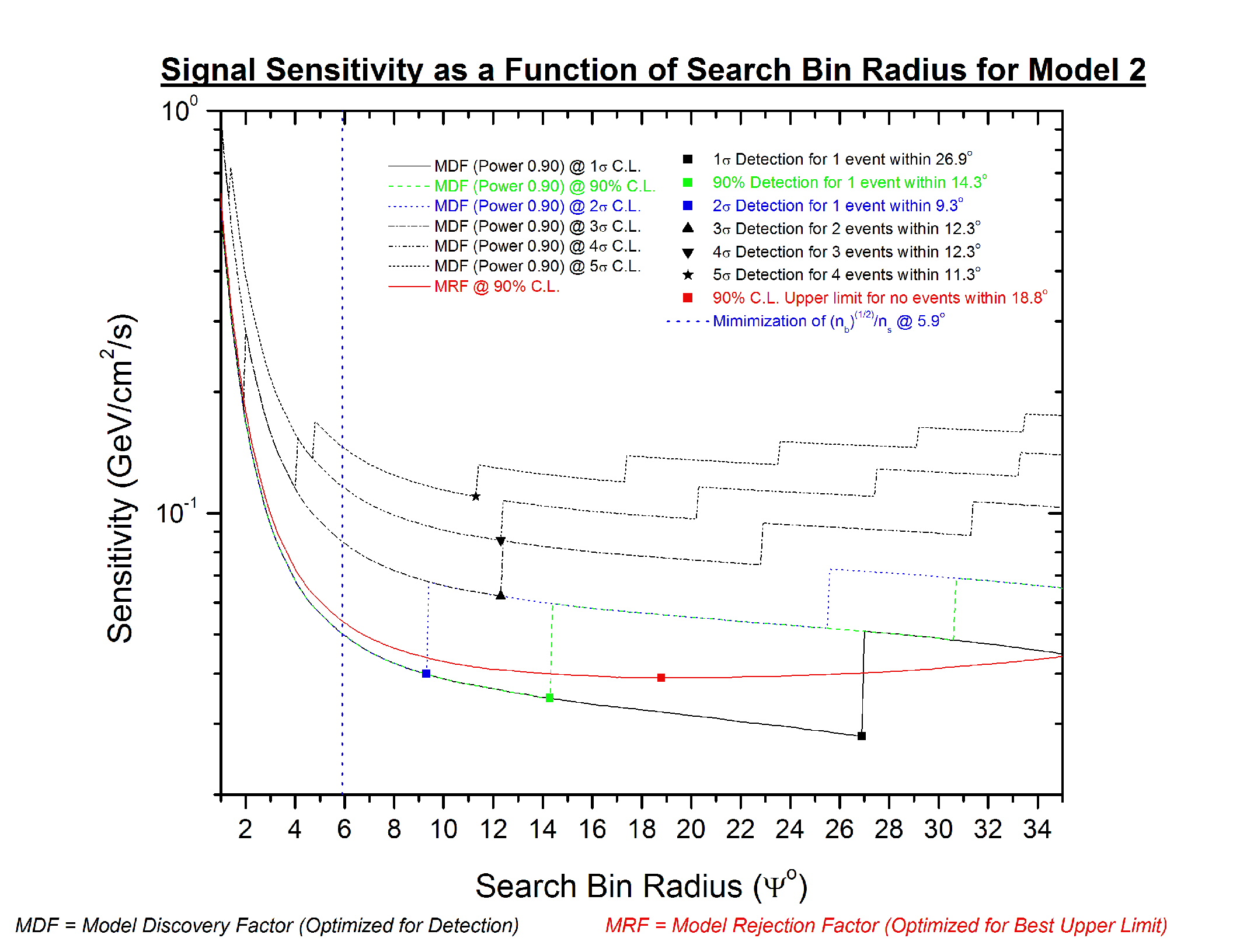
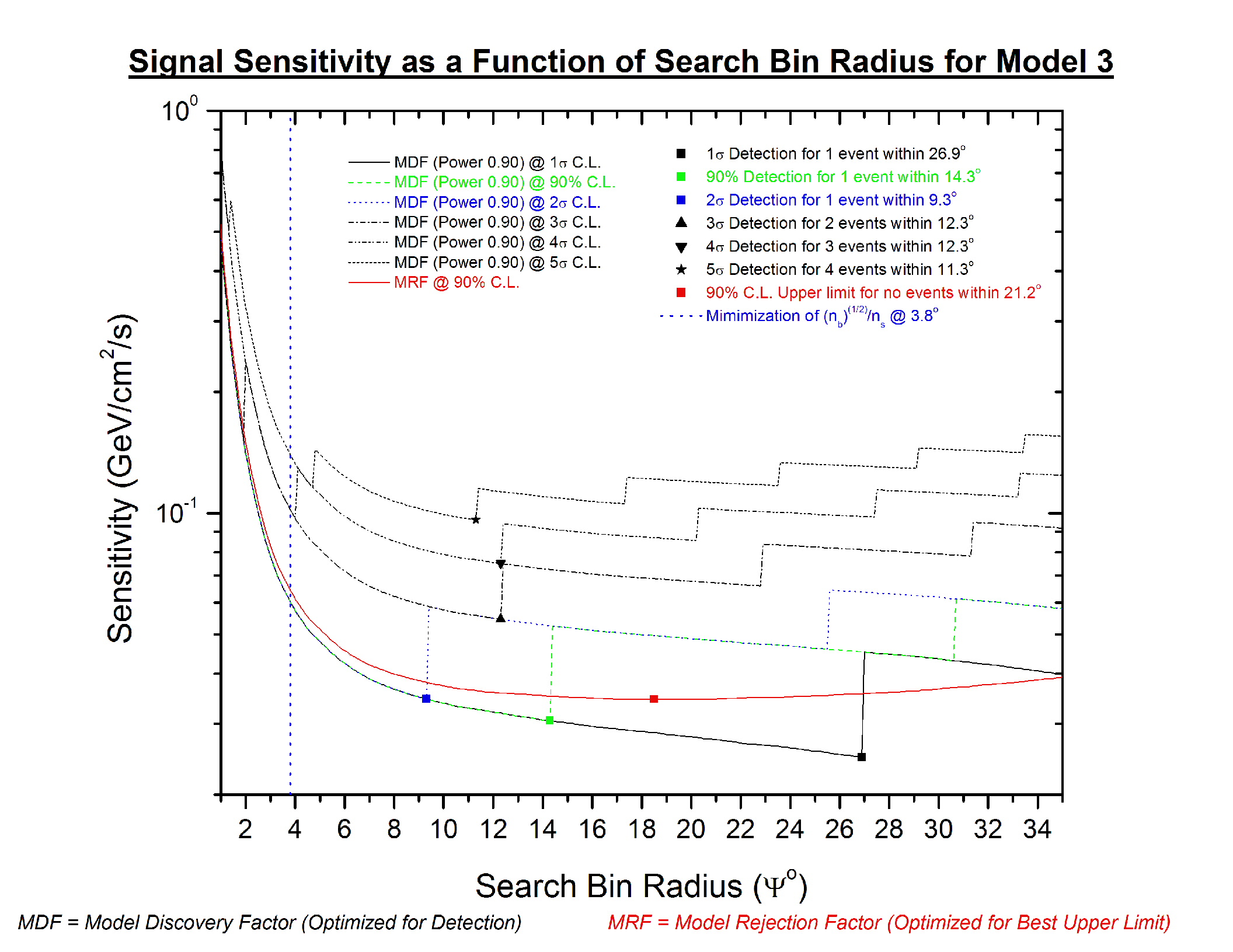
Preliminary investigations have shown that
global minimum of the MDF is independent of the statistical power, as
illustrated below. Hence a
constant power of 0.90 is used in all models.
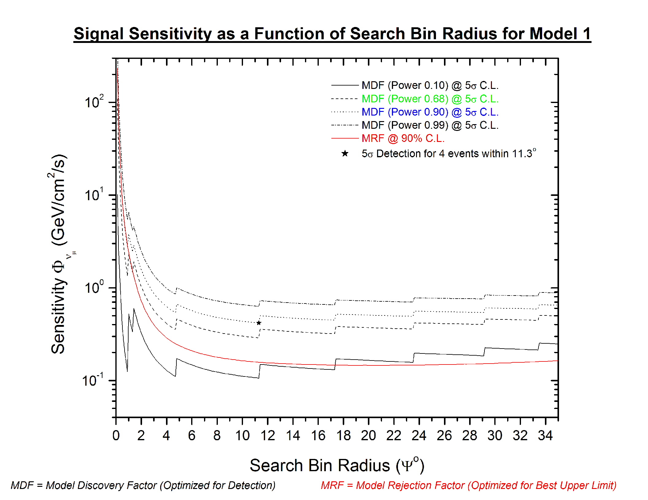
It should be noted that the MRF minimization is slightly different from before since we (i) have used an order of magnitude better resolution in the binning and no longer require a threshold trigger multiplicity of nch >= 24, since there was no software retriggering in the data set. The legend of each plot above reveals the line style and color code used throughout. The points represent the location of the global minimum for each optimization curve. Discussions have lead to a consensus of 5 sigma detection for a claim of discovery, which amounts to a cut at 11.3 degrees. Using a fixed statistical power of 90, we noted that one looses ~5-8% in limit setting potential when moving from a cut optimized for MRF minimization (~18-20 degrees) to a cut based upon the minimum MDF for the 5 sigma curve (11.3 degrees). However, one gains a reduction of ~17-26 degrees in the minimum flux required to satisfy the discovery criterion.
| Neutrino | Maximum Search | Background | Signal | Model Rejection Potential (MRP) | Model Discovery Potential (MDP) | ||||||||
| Flux | Bin Radius | nb | ns | 90% C.L. | Sensitivity | 90% C.L. | 0.90 Power @ 5s | Sensitivity | 0.90 Power @ 5s | ||||
| Model | Y (°) | Integrated | Integrated | m90 | MRF | FnmL (GeV/cm2/s) | Dm90 (%) | DMRF (%) | m90' | MDF | FnmD (GeV/cm2/s) | Dm90' (%) | DDFF (%) |
| 1 | 11.3 | 0.061401 | 0.0156259 | 2.49158 | 159.451 | 0.157218686 | -5.6 | 7.3 | 6.6196 | 423.629 | 0.417698194 | -36.7 | -19.9 |
| 21.3 | 0.228161 | 0.0178074 | 2.63165 | 147.785 | 0.14571601 | 5.3 | -7.9 | 9.04684 | 508.039 | 0.500926454 | 26.8 | 16.6 | |
| 2 | 11.3 | 0.061401 | 0.00924695 | 2.49158 | 269.448 | 0.041494992 | -3.8 | 6.0 | 6.6196 | 715.868 | 0.110243672 | -37.5 | -24.5 |
| 18.8 | 0.173737 | 0.0102128 | 2.58594 | 253.207 | 0.038993878 | 3.6 | -6.4 | 9.10126 | 891.166 | 0.137239564 | 27.3 | 19.7 | |
| 3 | 11.3 | 0.061401 | 0.000613275 | 2.49158 | 4062.74 | 0.036280268 | -3.6 | 5.0 | 6.6196 | 10793.8 | 0.096388634 | -37.6 | -26.2 |
| 18.5 | 0.167457 | 0.000668527 | 2.58066 | 3860.23 | 0.034471854 | 3.5 | -5.2 | 9.10754 | 13623.3 | 0.121656069 | 27.3 | 20.8 | |
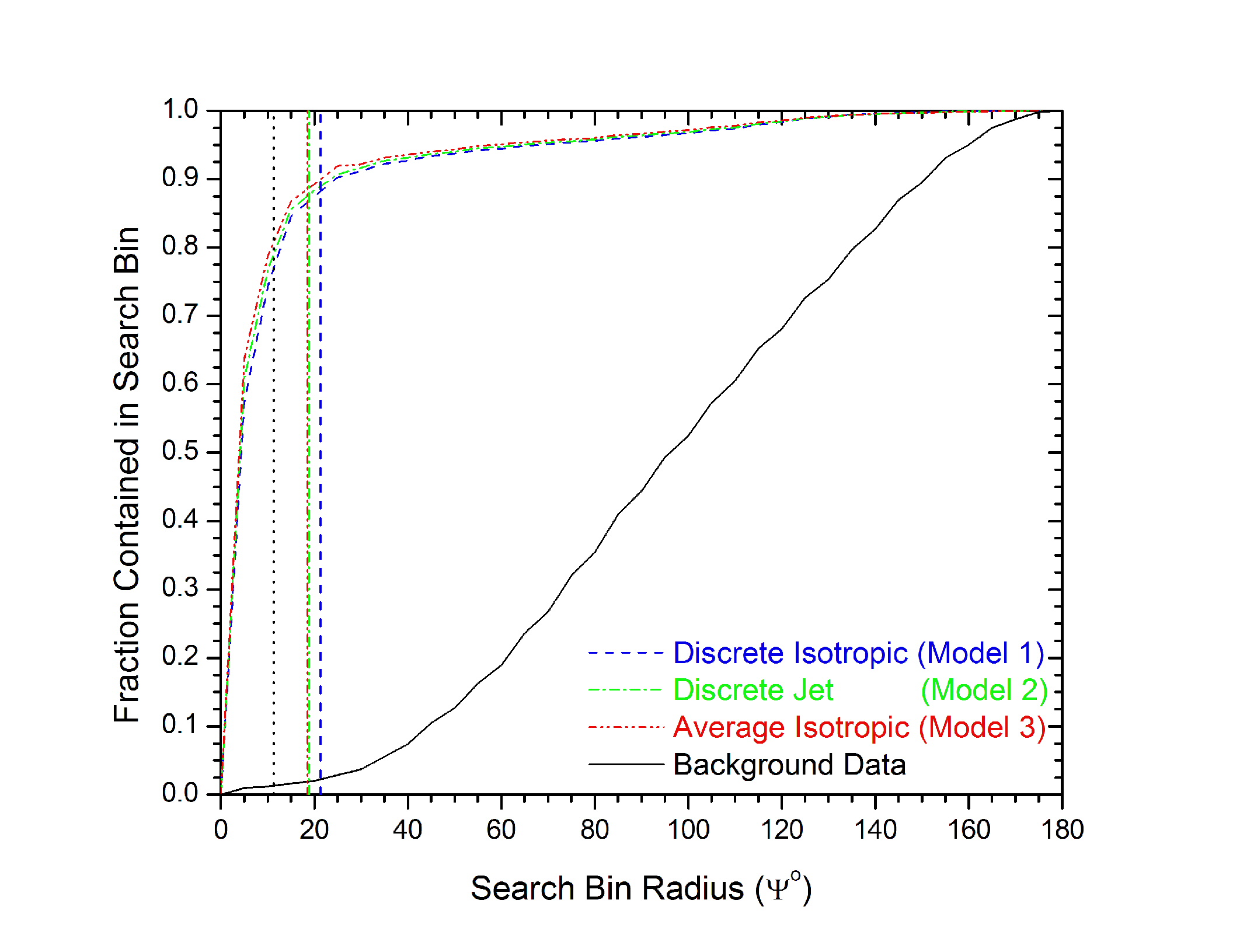
Since we gain more than we loose (due tot eh relative shallow minimum of the MRF curve) we decided optimize the cuts for discovery, i.e. the maximum search bin radius was taken as 11.3 for all models, with an on-time search window of 40 seconds. This is still relatively robust, since both the MRF and MDF optimized search bin radii reject ~99% of the background while retaining ~86% and ~77% of the signal, respectively, as illustrated below:
These results should be discussed on a collaboration wide level, since it makes sense to keep optimization uniform across analyses, e.g. how does this impact the diffuse GRB search? Does it make sense for one GRB analysis to be discovery based while another is going for the best limit?
8. Results
The expected number of background events in the 40 second on-time interval was ~17 events. Looking on-time lead to the observation of 15 events, which is a bit lower than expected, but within statistical uncertainty. A search bin radius cut at 11.3 degrees removed all events. Hence no events were observed on-time. The final flux upper limits are given below, note that we only report a ~5% higher limit than we would have if the MRF cuts were chosen.
| Neutrino | Maximum Search | Background | Signal | Events | Model Rejection Potential (MRP) | |||||
| Flux | Bin Radius | nb | ns | Observed | 90% C.L. | Limit | 90% C.L. | Limit | ||
| Model | Y (°) | Integrated | Integrated | nobs | m90 | MRF | FnmL (GeV/cm2/s) | Dm90 (%) | DMRF (%) | DFnmL (GeV/cm2/s) (%) |
| 1 | 11.3 | 0.061401 | 1.56E-02 | 0 | 2.37 | 152 | 0.149547866 | -5 | -5 | -5 |
| 2 | 11.3 | 0.061401 | 9.25E-03 | 0 | 2.37 | 256 | 0.039470312 | -5 | -5 | -5 |
| 3 | 11.3 | 0.061401 | 6.13E-04 | 0 | 2.37 | 3864 | 0.034509967 | -5 | -5 | -5 |
The following table is taken from the ICRC proceedings:
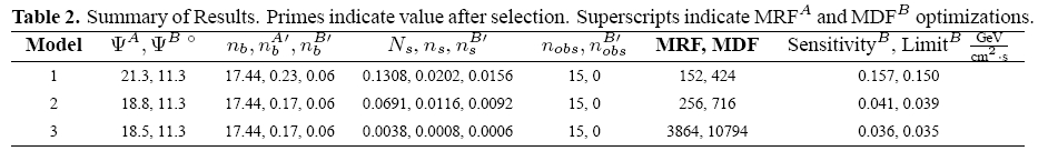
Where: the superscripts A and B refer to either MRF or MDF optimization method, respectively.
nb = number of expected background events
Primed variables indicate values after cut has been applied
nobs = Number of observed events on-time
Ns = Number of events in IceCube
ns = Number of events in AMANDA_II