Multipole Analysis - Method
Introduction/Reminder
Notice: In order to understand how the skymaps of this chapter are simulated also read the chapter Simulation of the Skymaps.
Parameters used in this chapter include:
- \(\mu\): Average Source Strength - Equivalent to the average amount of neutrinos from one source (\(\mu_{tot}\) for all years, \(\mu_{IC79}\) only IC79)
- \(N_{Sou}\): Number of Sources
- \(<n_{s}>=\mu_{tot} \cdot N_{Sou}\): Expected overall amount of signal neutrinos
Spherical harmonics
General relations
Every neutrino event has a fixed position on a skymap described by two coordinates: zenith angle \(\theta\) and azimuth angle \(\phi\). An example of such a skymap, as it is used in this analysis, is shown in the plot below.
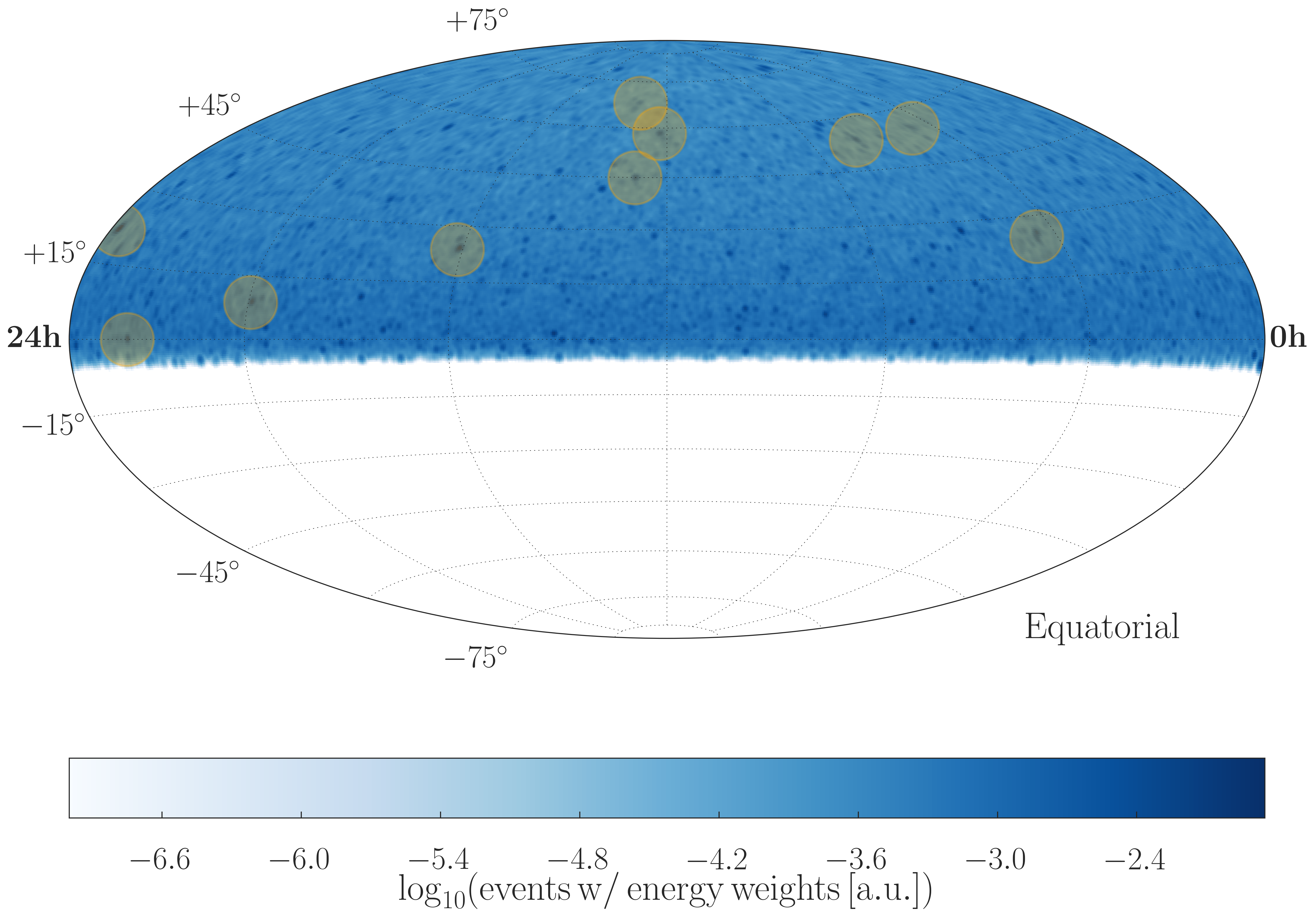
Fig. 1 Exemplary Experiment Like Skymap with 10 Sources and \(\mu_{tot}=34.2\)
The idea is now to use the fact that any distribution on a sphere can be expanded into spherical harmonic functions \(Y_{l}^{m}(\theta, \phi)\). This is possible, because spherical harmonics form a full set of orthonormal functions and therefore fulfill the following relations:
Orthogonality and normalization:
\(\int _{0}^{2\pi} d\phi \int _{0}^{\pi} d\theta \sin (\theta) Y_l ^{*m} (\theta, \phi) Y_{l'} ^{m'}(\theta, \phi) = \delta_{ll'} \delta_{mm'}\)
Completeness:
\(\sum _{l=0}^{\infty} \sum_{m=-l}^{l} Y_l ^{*m}(\theta, \phi) Y_l ^{m}(\theta', \phi') = \delta (\Omega-\Omega')\), where \(d\Omega=\sin(\theta)d\theta d\phi\)
They are constructed to form solutions to the angular part of the Laplace equation \(\Delta f(r, \theta, \phi) = 0 \Rightarrow f(r, \theta, \phi) = R_l(r) \cdot Y_l ^{m}(\theta, \phi)\), where ‘’R’’ denotes the radial and ‘’Y’’ the angular solution. Spherical harmonics can be expressed using the ‘’associated Legendre polynomials’’ \(P_{lm}\) and a normalization constant:
\(Y_l ^{m}(\theta, \phi) = N_{lm} \cdot P_{lm} \cos(\theta) \cdot \exp(im\phi)\)
More information about Legendre polynomials can be found here. In general a function on a sphere (=with constant radius) can be written with spherical harmonics and coefficients \(a_l^m\):
\(f(\theta, \phi)= \sum_{l=0}^{\infty} \sum_{m=-l}^{l} a_l ^m Y_l ^m (\theta, \phi)\), where \(a_l ^m = \int _{0}^{2\pi} d\phi \int _{0}^{\pi} d\theta \sin (\theta) Y_l ^{*m} (\theta, \phi) f(\theta, \phi)\)
When now the second part is plugged in the first part it yields
\(f(\theta, \phi)= \sum_{l=0}^{\infty} \sum_{m=-l}^{l} \left( \int _{0}^{2\pi} d\phi \int _{0}^{\pi} d\theta \sin (\theta) Y_l ^{*m} (\theta, \phi) f(\theta, \phi) \right) Y_l ^m (\theta, \phi)\)
Integral and sum can be swapped and the completeness relation then gives \(f(\theta, \phi) = \int d\Omega \delta (\Omega-\Omega') f(\theta', \phi') = f(\theta, \phi) \checkmark\)
Implementation
This analysis uses the healpy package to create and analyze skymaps. It provides a function (anafast()) which returns \(a_l ^m\) and the corresponding power coefficients \(C_l\) (see next sub item) for one map up to a given limit \(l=l_{\mathrm{max}}\). The limit in this analyis is chosen to be \(l_{\mathrm{max}}=1000\), a value that is high enough that the \(a_l ^m\) values resemble the whole map up to its finite resolution (see figure below). The implementation can now be understood in terms of the theoretical relations explained above. A map with a given number of N events is a sum over delta distributions, multiplied by a energy weighting factor in order to respect the different energy distributions of conventional and astrophysical neutrino fluxes (see sec. Energy Weights ).
\(f_{\mathrm{map}}(\theta, \phi) = \sum _{i=1}^N c_i \cdot \delta(\theta-\theta_i) \delta(\phi-\phi_i)\)
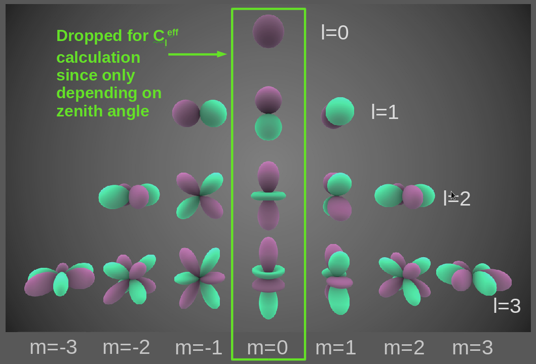
Fig. 2 Visual representations of the first 4 bands of real spherical harmonic functions. Purple portions are regions where the function is positive, and green portions represent regions where it is negative.
\(C_{l}^{eff}\) spectra
The expansion coefficients contain all information of a skymap up to a given resolution coded in angular relations between all points (hence the name ‘’angular auto-correlation analysis’‘). The information of event clustering on a certain angular scale is contained in the (effective) power spectrum \(C_l\) defined as
\(C_l = \frac{1}{2l+1} \sum _{m=-l}^{l} \left| a_l^m \right| ^2\)
Directional dependence of \(a_l ^m\) coefficients is canceled out by using the absolute square. It is convenient to average over all \(m\) for each \(l\) to get to a spectrum which only depends on the angular distance \(\alpha\) (\(180/l~\alpha\)) between events. In this particular analysis an effective power spectrum is used, meaning that all coefficients \(a_l ^{m=0}\) are discarded from the sum. Since these coefficients are purly zenith dependent, this results in a small loss of information, but reduces the zenith dependent systematic errors significantly. Hence the effective power spectrum is defined as
\(C_l^{eff} = \frac{1}{2l} \sum _{m=-l, m\neq 0}^{l} \left| a_l^m \right| ^2\)
After simulating a larger amount of skymaps (in general 1.000 or 10.000 in this analysis) the stastical mean and error on \(C_l^{eff}\) is calculated for each \(l\) (see plot beneath). This yields an overall averaged spectrum with a statistical error \(\sigma_l\) on each coefficient which is needed for further calculations, e.g. the test statistic \(D^{2}_{eff}\) as it is explained in the next section.
An example of such a power spectra is shown below. It’s obvious (and of course just logical) that there is a strong correlation between the lines for different number of sources. A more careful investigation shows that the spectra scale with a linear coefficient plus and an offset. The offset is here given by the continous shift from zero for pure background maps (\(N_{Sou}=0\)). After subtracting the offset from the distributions the linear scaling coefficient can be calculated by just taking the ratio for each point. This ratio-distribution including the mean value are shown in the second plot. The mean value is in good agreement with the ratio of the number of sources.
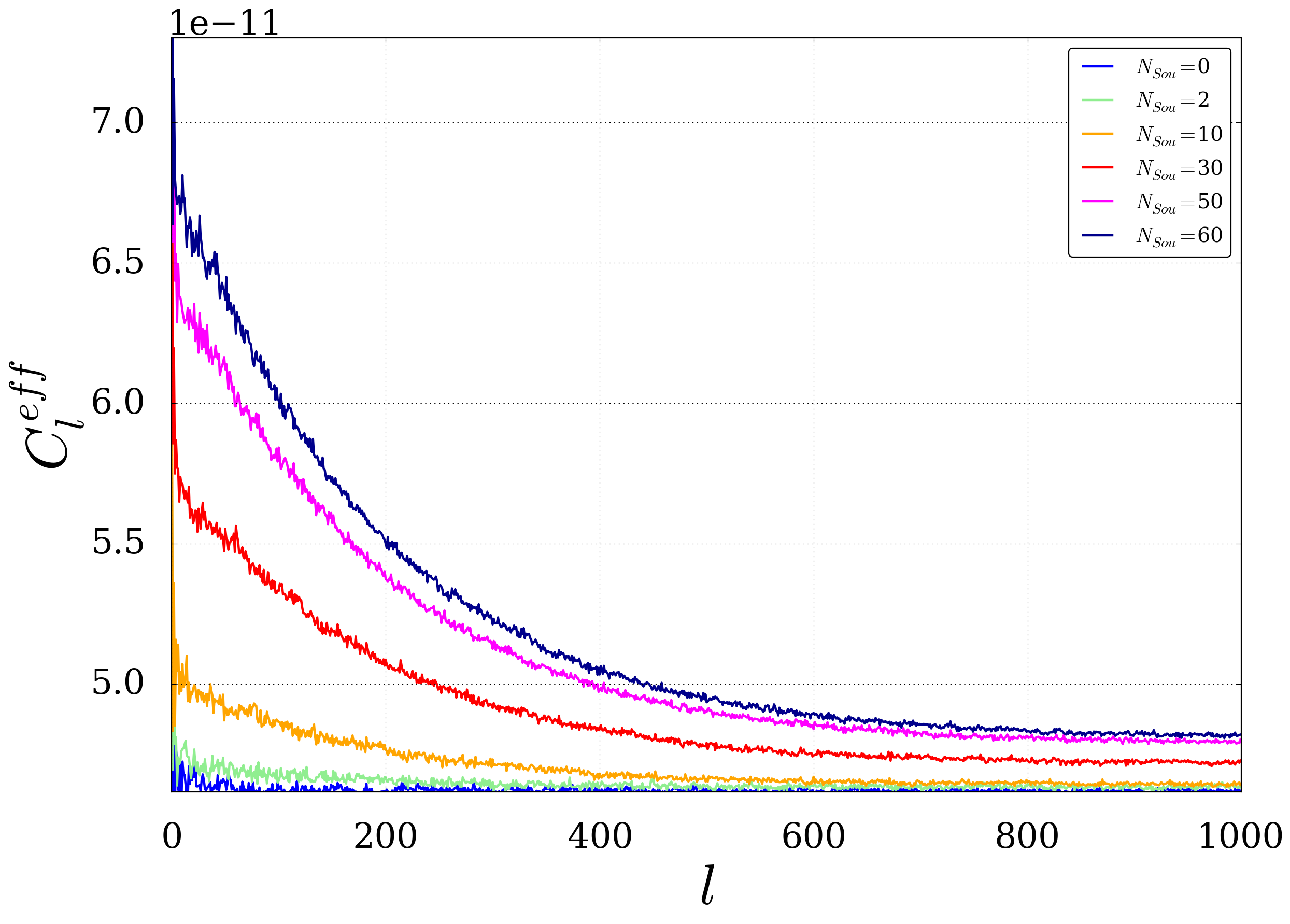
Fig. 3 The plot shows the statistical mean of a power spectra \(C_l^{eff}\) calculated from 1.000 Experiment-Like Skymaps with \(\mu_{tot}=8.55\)
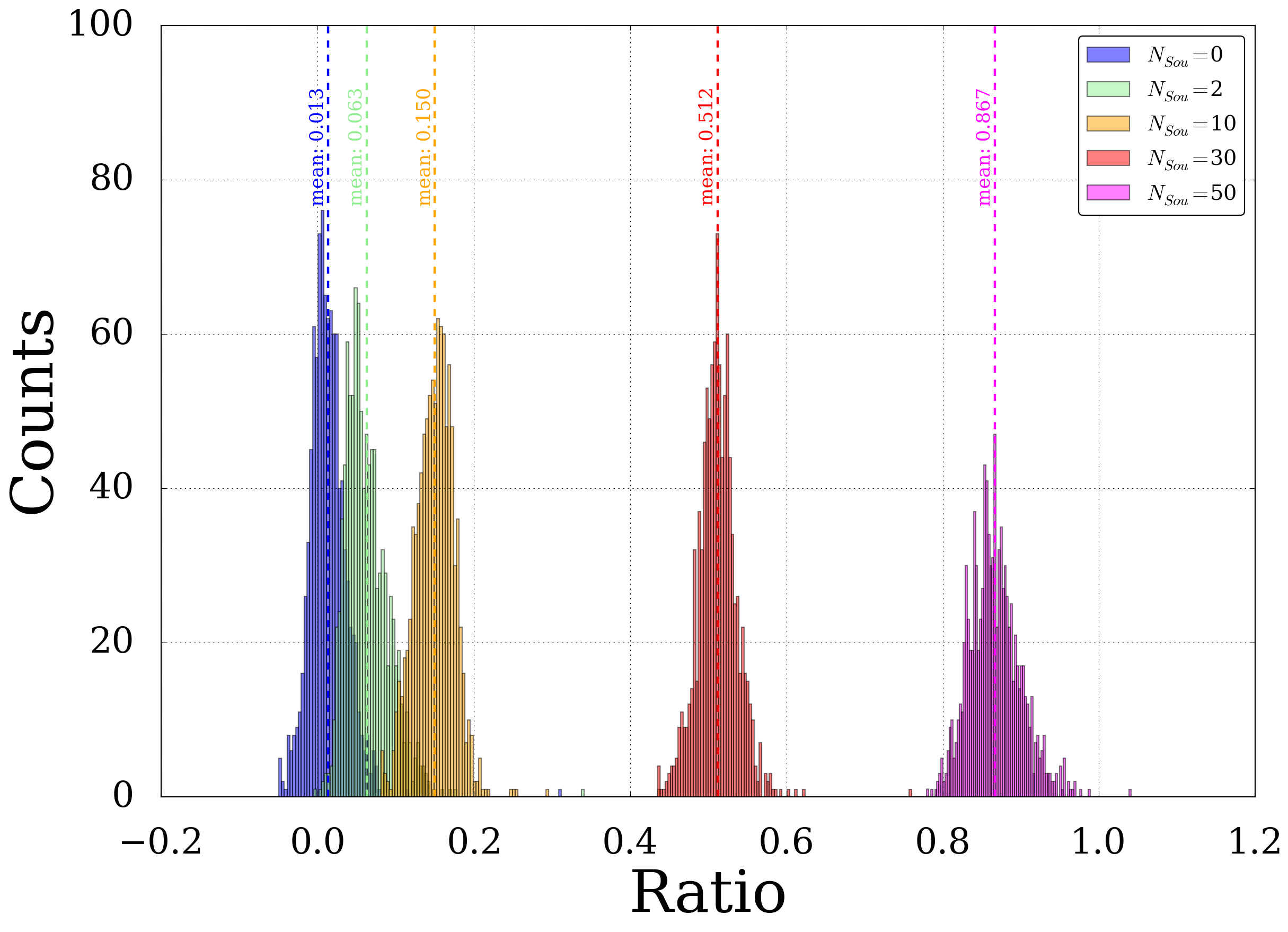
Fig. 4 Ratio of the linear scaling coefficient \(C_l^{eff}(N_{Sou}) \mathbin{/} C_l^{eff}(N_{Sou}=60)\)
Re-normalization
When comparing scrambeled experimental data with the MC simulated BG maps we find a systematic shift of both test statistic distributions. This is caused by the fact, that the scrambled experimental maps are already one possible realisation of the background hypothesis. But in contrast to the MC simulated background maps the events for the scrambled experimental map are highly correlated for each skymap. As a result we would already measure a TS shift (and therefore a significance \(\Sigma \neq 0\)) even if our real experimental skymap is completly diffuse. A detailed analysis has been performed for the previous IC79 multipole analysis .
In order to match the simulated background maps and the scrambled experimental data a renormalization of the power spectra is applied. Renormalization means here, that the \(C_l^{eff}\) are transformed according to:
\(C_l^{eff} \rightarrow \frac{C_l^{eff}}{\sum_{l=0}^{l_{max}}C_l^{eff}}\)
The procedure is justified, because the information about the clustering is mainly encoded in the spectrum’s shape, not in it’s absolute value. The absolute value strongly depends on the specific configuration (zenith values, event energies) of the skymap and is therefore different for each simulation process and contributes to a larger statistical error on the power spectras mean value. In contrast to that for 1000x scrambled experimental maps the zenith and energy values which are used are the same for each skymap. This results in a systematic shift between the TS distributions of experimental maps compared to simulated background maps as explained above.
The first plot below shown an example of a renormalized power spectrum. As a result of the normalization all the lines cross in one point. Using a more detailed calculation this point \(l_0\) can be shown to coincide with the point where
\(\int_{0}^{l_{max}} C_l^{eff}(y) \mathrm{d}y = C_l^{eff}(l_0)\cdot(l_{max}-l_{min})\)
for any of the distributions
The second plot shows the good compliance of the scrambled background with simulated background maps (already using the fitting function explained below)
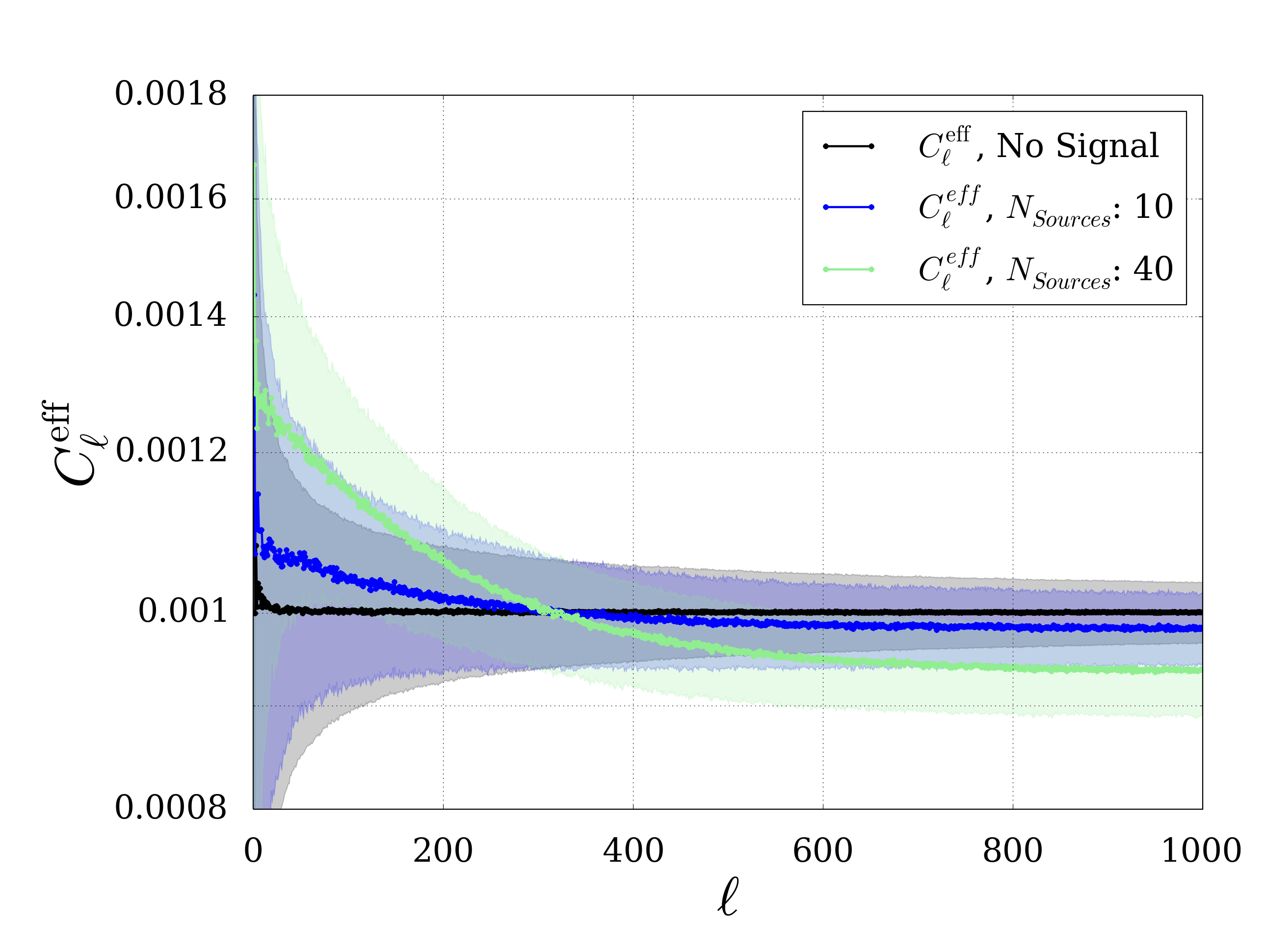
Fig. 5 Example for a renormalized power spectrum. The shaded areas show the statistical error, i.e. the standard deviation from the distribution for each l
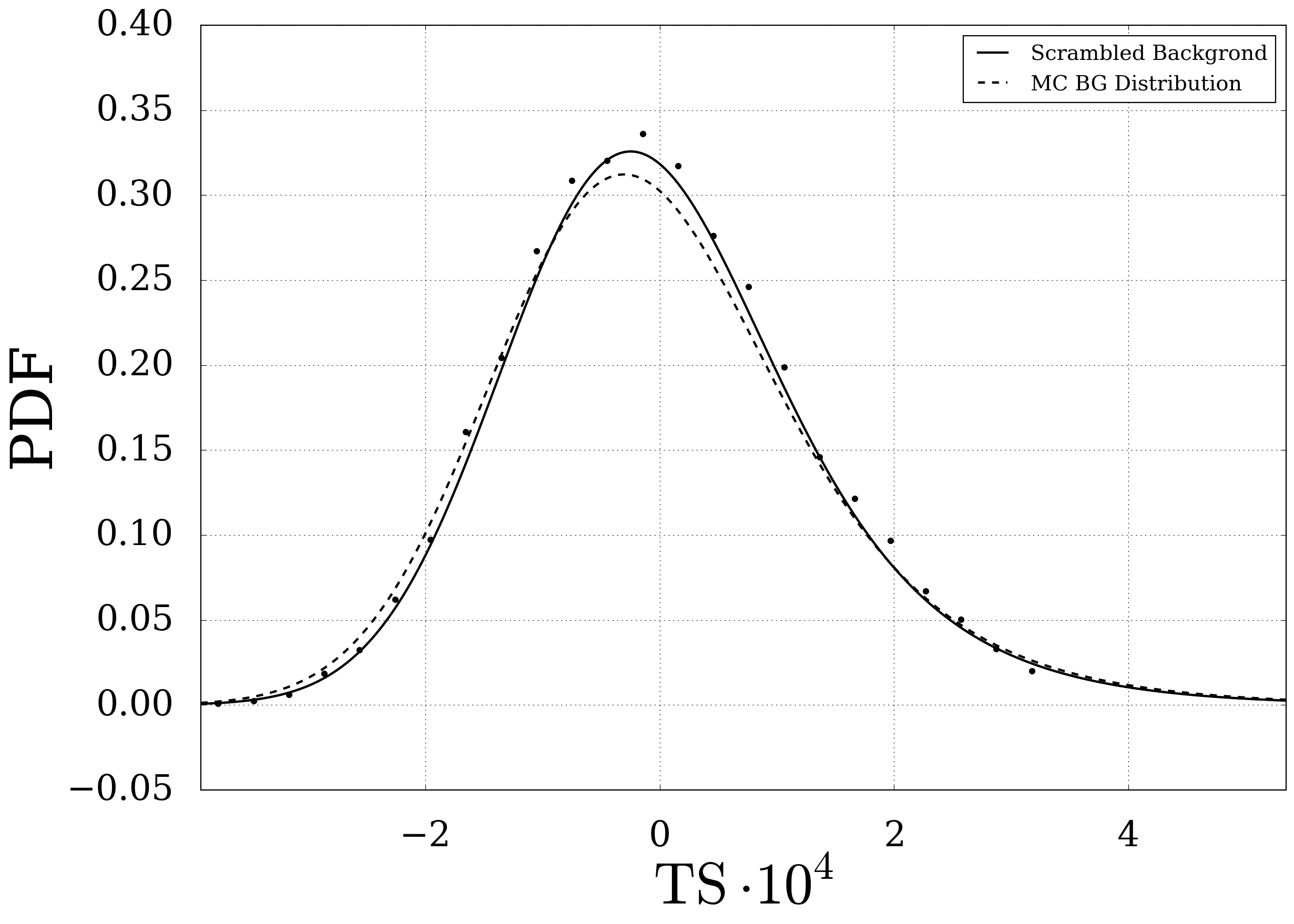
Fig. 6 Test statistic distribution for scrambled (solid) and simulated background maps (dotted).
Test statistic \(D^{2}_{eff}\)
Weights
The next step is to quantify the difference between signal and background. A first approach could be a \(\chi^2\) test for each signal/experimental map vs. averaged background.
\(\chi^2_{eff}=\sum_{l=1}^{l_{\mathrm{max}}} \left( \frac{C_{l, exp}^{eff} - \langle C_{l, bg}^{eff} \rangle}{\sigma_{l,bg}} \right)^2\)
This procedure is motivated by the fact that the background \(C_l^{eff}\) follow a nearly gaussian distribution in the relevant l range (compare these plots) and would already yield acceptable results. However the test can be improved by including the known properties of the spectra. From the pure signal spectra it is known on which scales \(l\) the separation power is the strongest. Hence it is reasonable to include weights which are calculated from 10.000 signal and background maps. They are basically defined as the difference between the mean signal and the mean background divided by the statistical error on the background spectrum depending on scale factor \(l\):
\(w_l^{eff}= \frac{\langle C_{l, sig}^{eff} \rangle - \langle C_{l, bg}^{eff} \rangle}{\sigma_{l,bg}}\)
The plot on the bottom of the section shows the distribution of weights that were calculated from the power spectra for the combined samples. There is a peak for all distributions at about \(l\sim 50\) where the separation power is strongest. The smallest number of sources is equivalent to the highest number of neutrinos per source, hence the largest deviation from diffusely distributed events. They also have the smallest statistical fluctuations, so it is an reasonably motivated choice to use the weight distribution of \(N_{sou}=5\) for further calculations. Since the weight distributions obviously have a different normalization it is necessary to correct for that through a normalisation factor in the test statistic (next section). The weight distributions differs in shape from the (typical) shape of the spectral distribution , but this can be understood from the statistical error on each point which is large at first but decreases with \(l\). Additional investigations show that the ratio of one set of weights to another truly is a constant factor (except for statistical fluctuations).
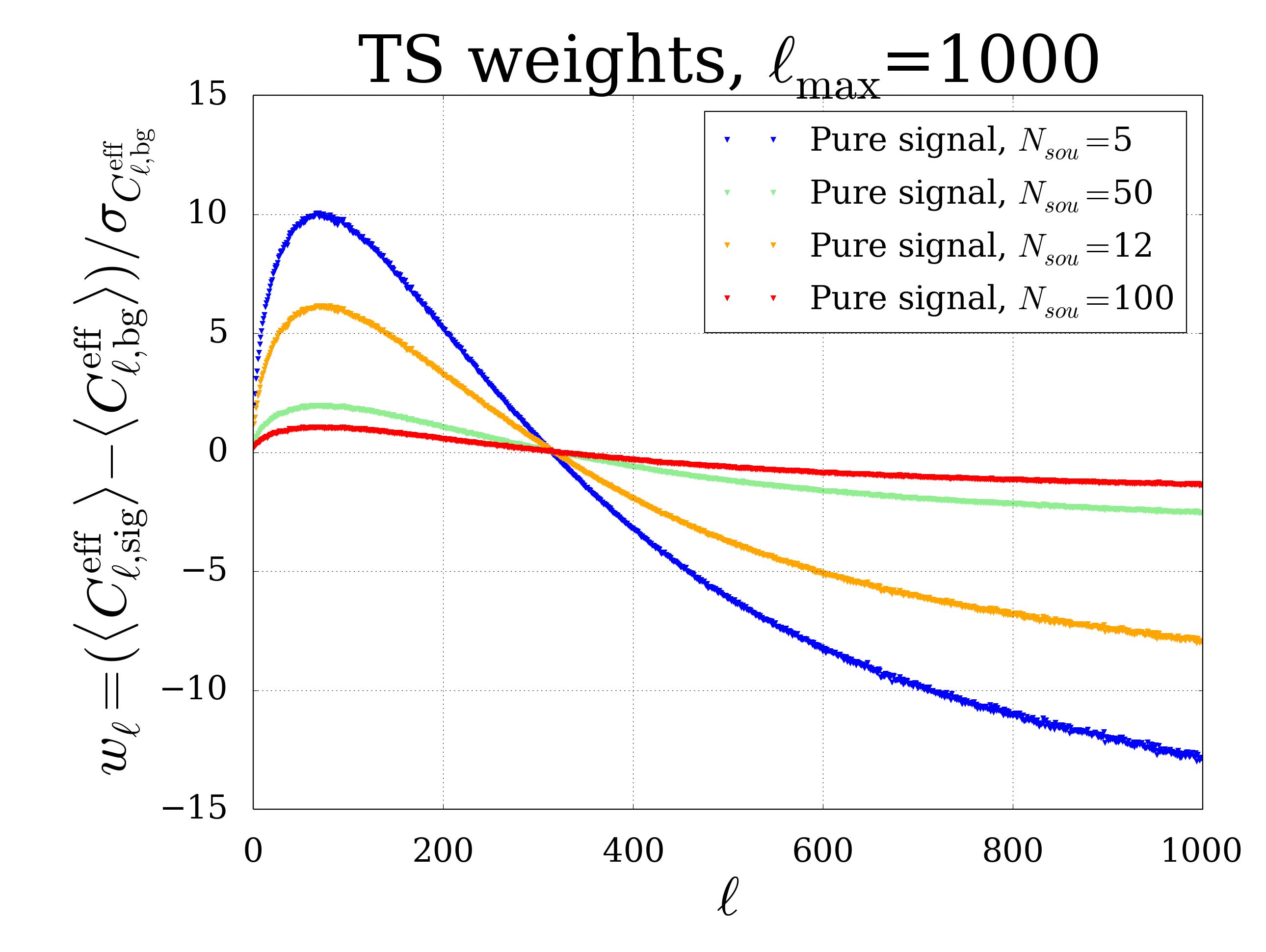
Fig. 7 TS weight distribution for different pure signal maps
Definition \(D^{2}_{eff}\)
Weights and \(\chi^2\) are combined to a single test statistic value \(D^{2}_{eff}\) for each map defined as
\(D^{2}_{eff}=\frac{1}{\sum_l w_l^{eff}} \cdot \sum_{l=1}^{l_{\mathrm{max}}} w_l^{eff} \left( \frac{C_{l, exp}^{eff} - \langle C_{l, bg}^{eff} \rangle}{\sigma_{l,bg}} \right)^2 \cdot \mathrm{sign}_l\)
where \(\mathrm{sign}_l\) denotes the sign of the difference of \(C_l^{eff}\) values. The standard procedure, where a \(\chi^2\) test is applied, does not care for the sign of deviations, but in this case it is important to know. Signal causes mainly positive deviations just as a lack of signal causes just statistically small deviations in both directions. Sign and value of the difference are equally important.
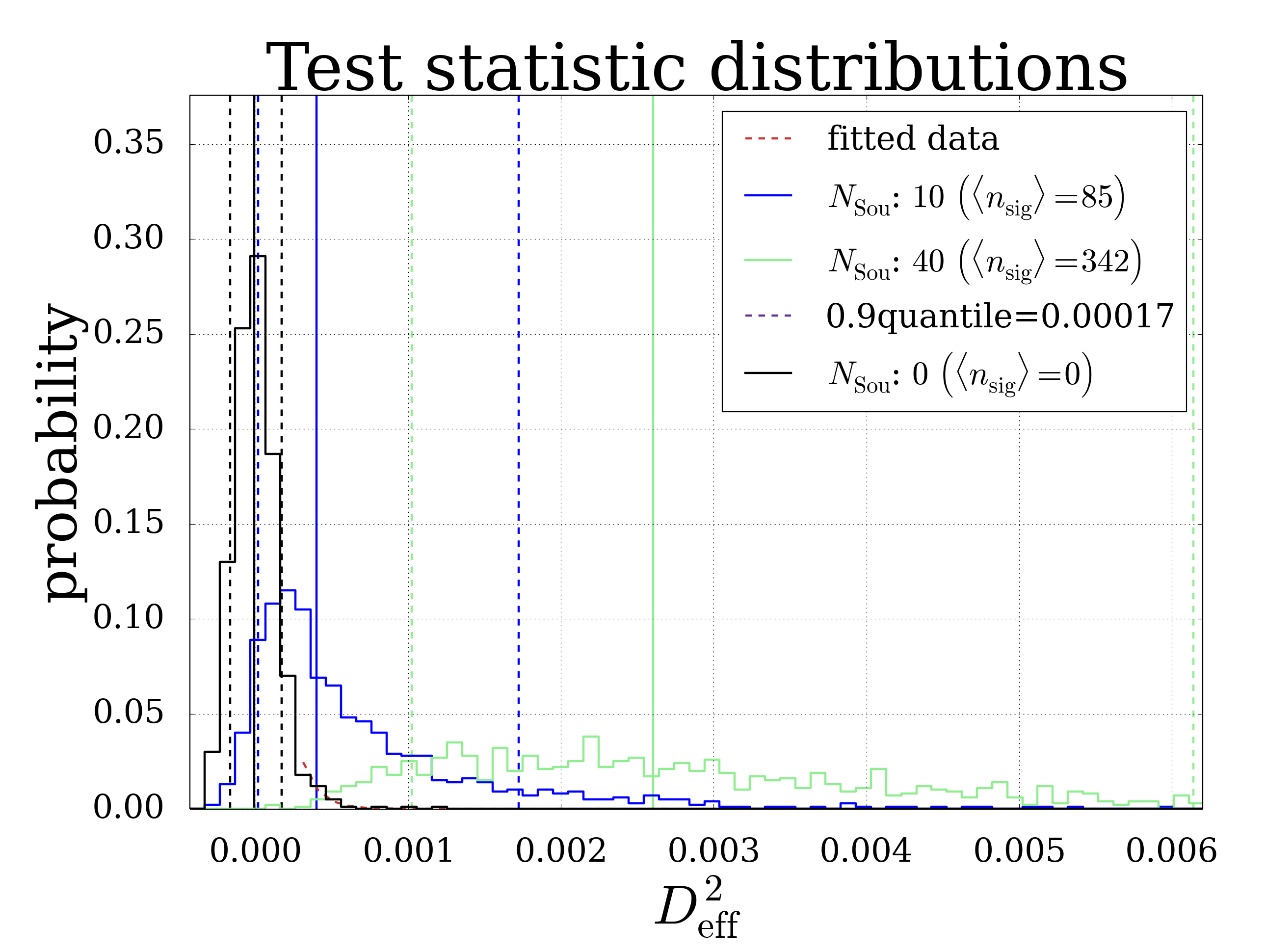
Fig. 8 Exemplary plot showing the test statistic distributions for different experimental like skymaps. For each ( \(\mu\) , \(N_{Sou}\) ) combination 1.000 skymaps have been simulated.
There is a plot of several \(D^{2}_{eff}\) distributions shown above. Single test statistic values are calculated for each signal map and then histogrammed to form the shown distribution. Vertical dashed lines in the same colors as the distributions indicate the median, the purple line indicates the 90%-quantile of the background. This distribution is simulated as experimental-like skymap with \(N_{sou}=0\) in order to get a measure of the spread of background distributions. It is visible that the black histogram doesn’t have a Gaussian shape, especially the tails are wider. This is important to account for when calculating the significance as explained in the next paragraph.
Significance
The significance is a measure for the shift of a skymaps TS value compared to the background distribution. For simulated skymaps we use the median of the corresponding TS distribution in order to get the minimum rejection power for the BG-only Hypothesis that we expect in 50% of the cases. For a symmetric distribution well described by a Gaussian shape the formula for the significance is rather simple:
\(\Sigma=\frac{\langle D^2_{eff, S} \rangle - \langle D^2_{eff, BG} \rangle}{\sigma_{D^2_{eff, BG}}}\)
However, as can be seen from the test statistics plots above, the probability density function (PDF) is not purely gaussian if energy weights are included in the analysis. In fact, the distribution developes a long stretched tail in addition to the gaussian shape around the maximum. Consequently a parametrisation with a superposition of a gaussian and anexponential function are used in the following. Two possible fit functions have been tested:
1.)
2.)
In the first case the fit parameters are \(\sigma,\,\mu,\,\mathrm{xcut}\,\mathrm{and}\,c\) and only those results assuring a continuous and (nearly) differentiable transition between the two regions, i.e. where the ratio \(f(xcut)/g(xcut)\approx 1\) are accepted. In the second case there is one fit parameter less. Hence we only have the 3 paremeters (\(\tau,\,\sigma\,\mathrm{and}\,t_0\)). The function basically describes a convolution of an exponential function with a gaussian. There is a slight modification (exponential term) in order to make the fit more stable. In each case the algorithm runs up to 1000 fit procedures and is implemented in a way, that it dynamically optimizes the starting conditions, i.e the number of fitted points, the fitting range, the fitting priors and the \(\chi^2\) giving it a maximum of stability and flexibility. In general the second functions appears to describe the distribution better and additionaly doesn’t have problems with non-differentiable points. An example for the Fit of the background distribution and of skymaps with source strength \(\mu_{tot}=3.42\) at \(\gamma=2.0\) is shown below for the convolution function of the gaussian and the exponential (2).
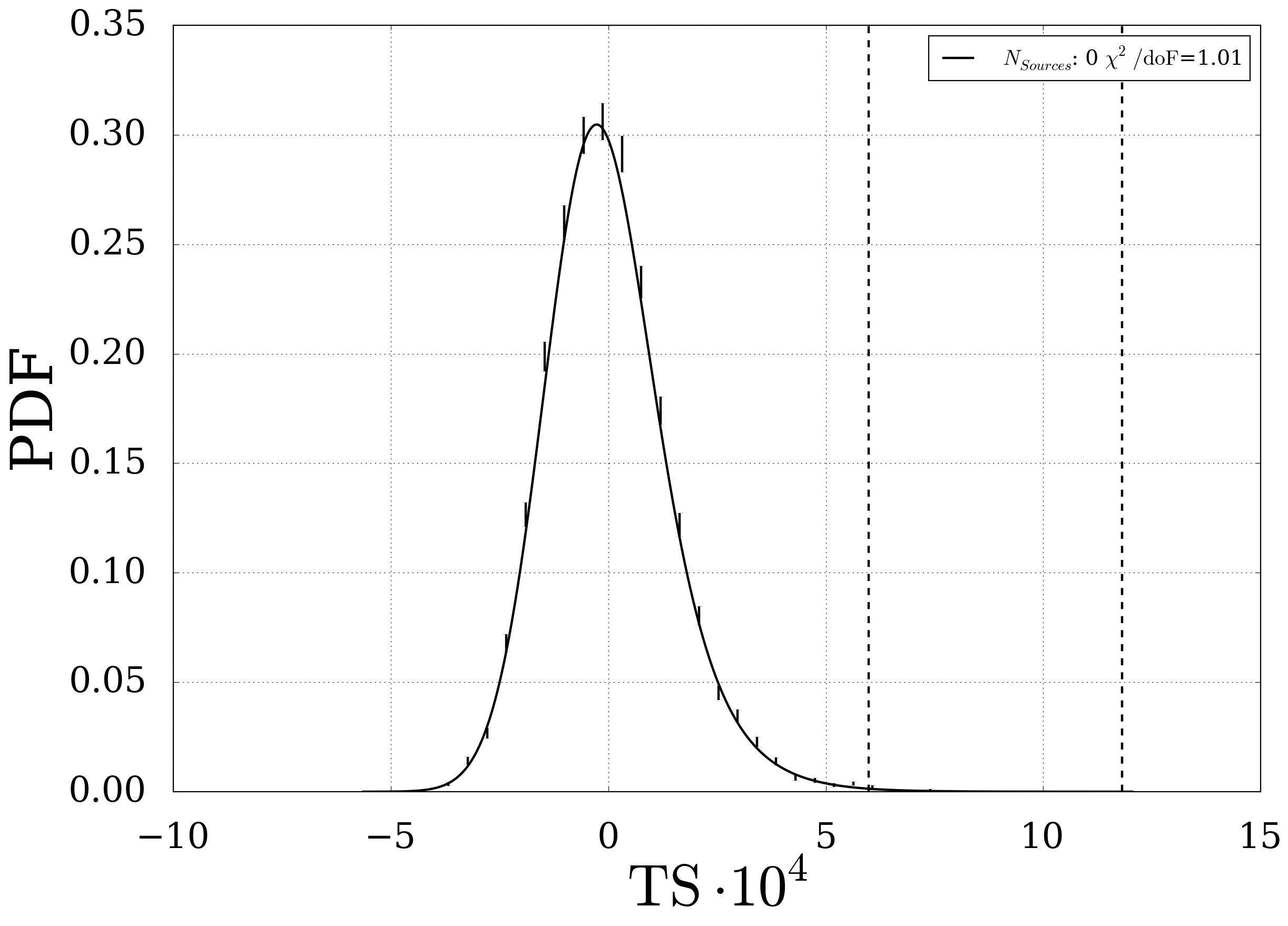
Fig. 9 Fit of the background distribution. The two dashed lines represent the one sided 3 and 5 sigma values of the TS.
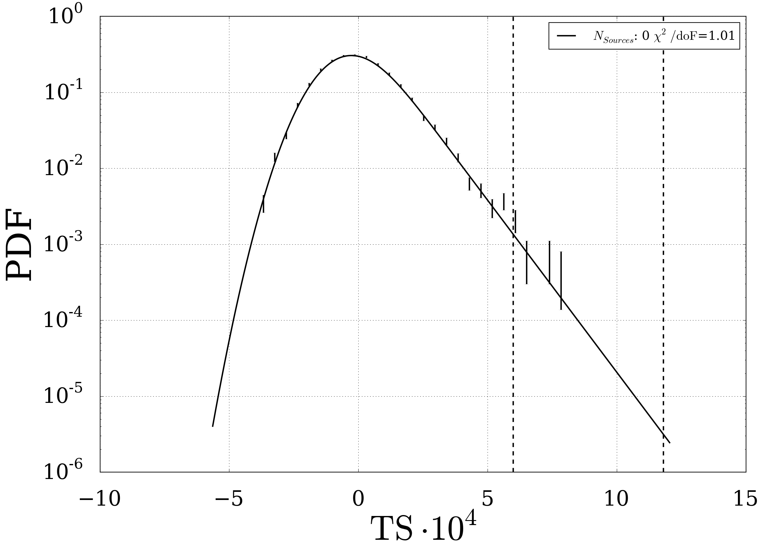
Fig. 10 The background distribution in logarithmic representation. The two dashed lines represent the one sided 3 and 5 sigma values of the TS.
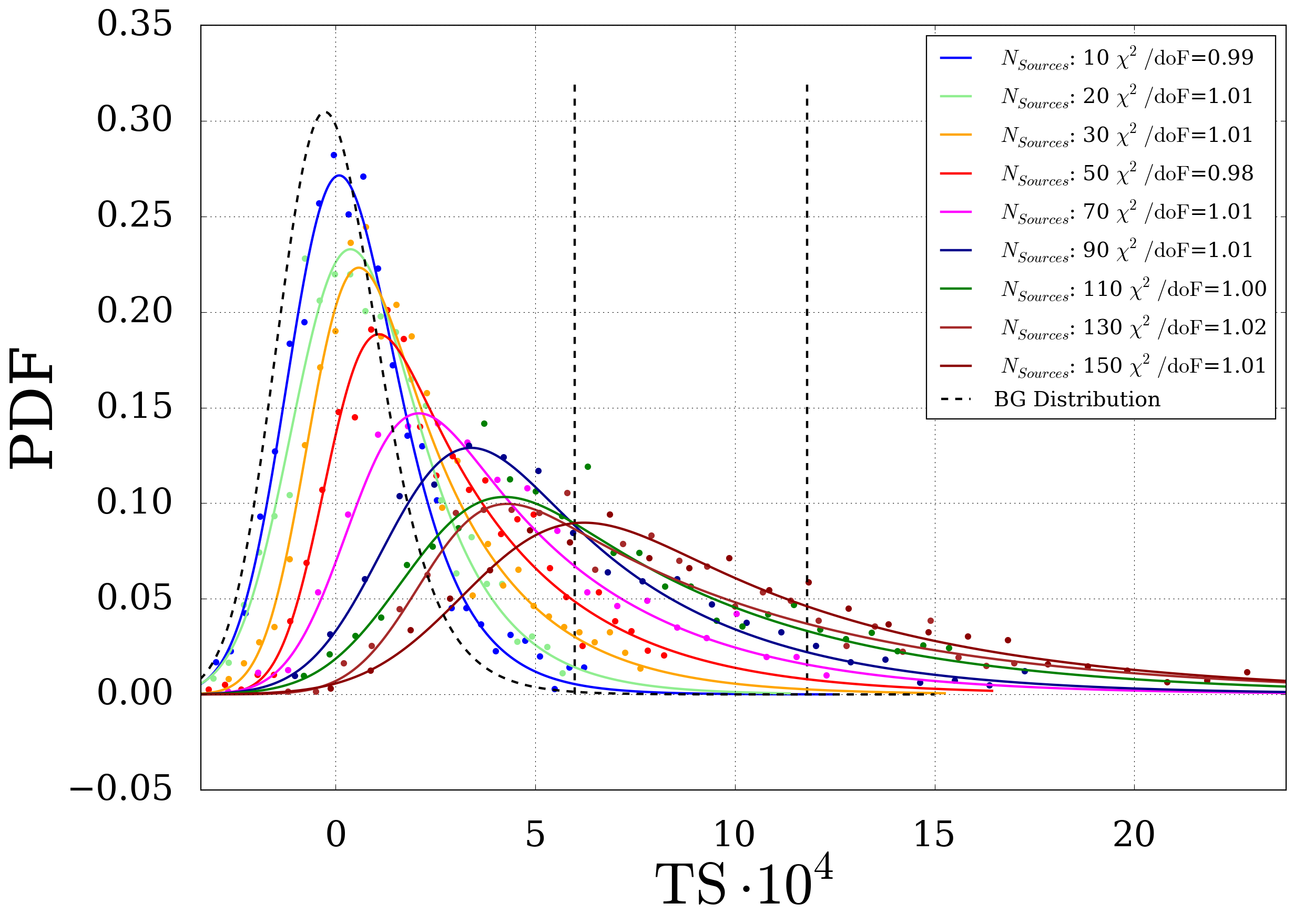
Fig. 11 Fit of the Signal Distribution for \(\mu_{tot}=3.42\) and different \(N_{Sou}\) using poissonian errors
Now the p-Value is calculated for each tuple of (\(\mathrm{N}_{Sou}, \mu_{tot}\)) using the test statistic median \(x_{median}\) from the signal distribution and evaluating the integral over the background \(PDF_{BG}(x=D^2_{eff,BG})\) at this position.
\(p=1-\int_{-\infty}^{x_{median}}PDF_{BG}(x) \mathrm{d}x\)
This can be translated to multiples of Gaussian standard deviation with the inverse error function and the convention \(q=1-p\)
\(\Sigma(\mu, N_{sou}) = \mathrm{erf}^{-1}(2q_{\mathrm{med}}(\mu, N_{sou})-1)\cdot \sqrt{2}\)
The significance is calculated for several sets of parameters and finally plotted in different ways:
- For fixed \(\mu_{tot}\) the significance is shown as the function of signal neutrinos \(n_s=N_{Sou} \cdot \mu_{tot}\)
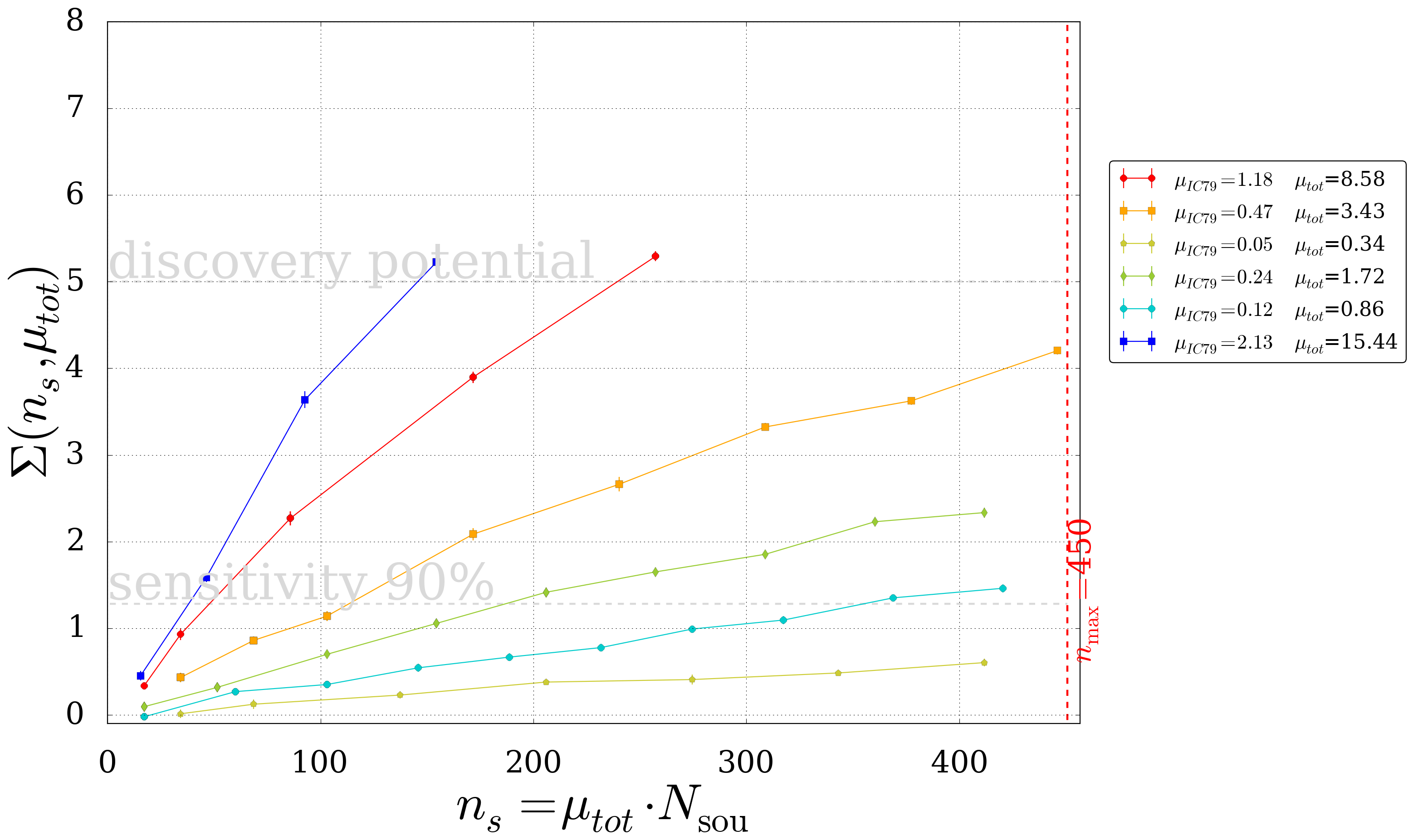
Fig. 12 The significance as a function of the number of signal neutrinos
- The parameter space for which the analysis is sensitiv is shown as shaded area. The dashed lines represent a fixed number of sources.
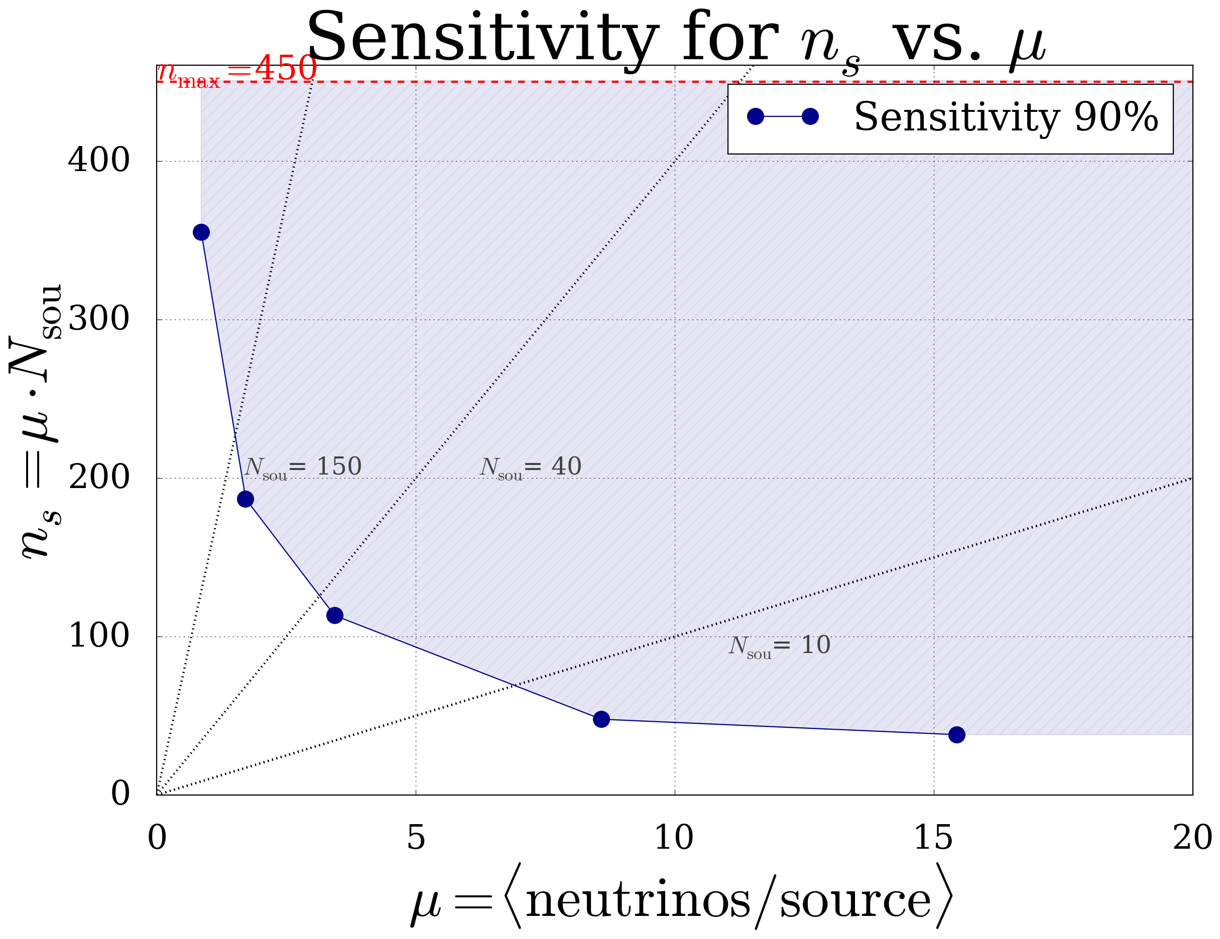
Fig. 13 Sensitiv parameter space of this analysis
- In order to compare the results to other analysis (Multipole IC79/Standard Point Source) the \(\mu_{tot}\) for which the analysis is sensitiv can be transformed into a ‘’Flux Normalisation per Source’’ (\(\Phi_{0}/N_{Sou}\)). The calculation is mainly based on the effective area of the detector in dependency of the energy. A corresponding plot is shown in the Supplementary Plots and Material section. The relation between the flux and a tuple \((\mu_{tot}, N_{Sou})\) is then \(\frac{1}{N_{Sou}}\frac{\mathrm{d}\Phi}{\mathrm{d}E}\cdot E^{\gamma}=\frac{\Phi_0}{N_{Sou}}=\frac{\mu}{\sum_{x \in \mathrm{samples}}T_x \cdot\int_{0}^{\infty}A_{\mathrm{eff,x}}\cdot E^{-\gamma}\mathrm{d}E}\). The plot below shows the Flux Normalisation per Source for different analysis methods. For further reference the best fit value from the diffuse fit is also included.
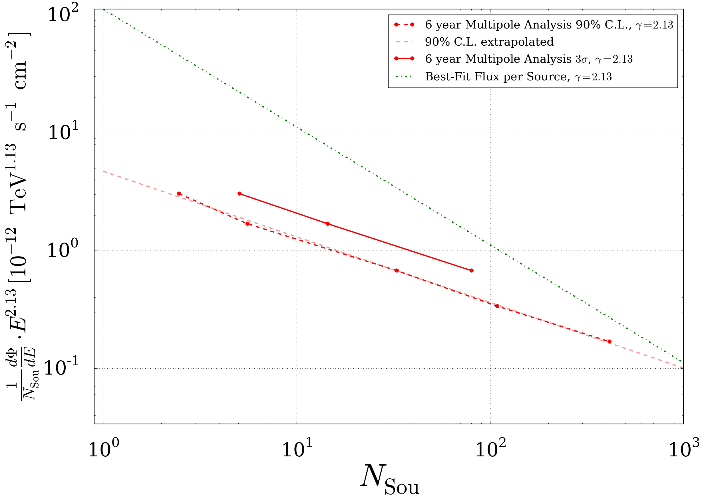
Fig. 14 Sensitivity comparison between different analysis methods