Performance

This section shows the performance results for different spectral indices \(\gamma\). In order to intepret the results from the sensitivity calculations for each parameter touple (\(N_{Sou}\), \(\mu\)) the corresponding flux normalisation per Source is calculated. The conversion makes use of the Detectors effective areas for each sample and is written as

\[\frac{1}{N_{Sou}}\frac{\mathrm{d}\Phi}{\mathrm{d}E}\cdot E^{\gamma}=\frac{\Phi_0}{N_{Sou}}=\frac{\mu}{\sum_{x \in \mathrm{samples}}T_x \cdot\int_{0}^{\infty}A_{\mathrm{eff,x}}\cdot E^{-\gamma}\mathrm{d}E}\]

Where possible the results form the Standard Point Source Analysis and the previous IC79 Multipole Analysis are also shown for comparison.

• \(\gamma=2.0\) (Benchmark Test)

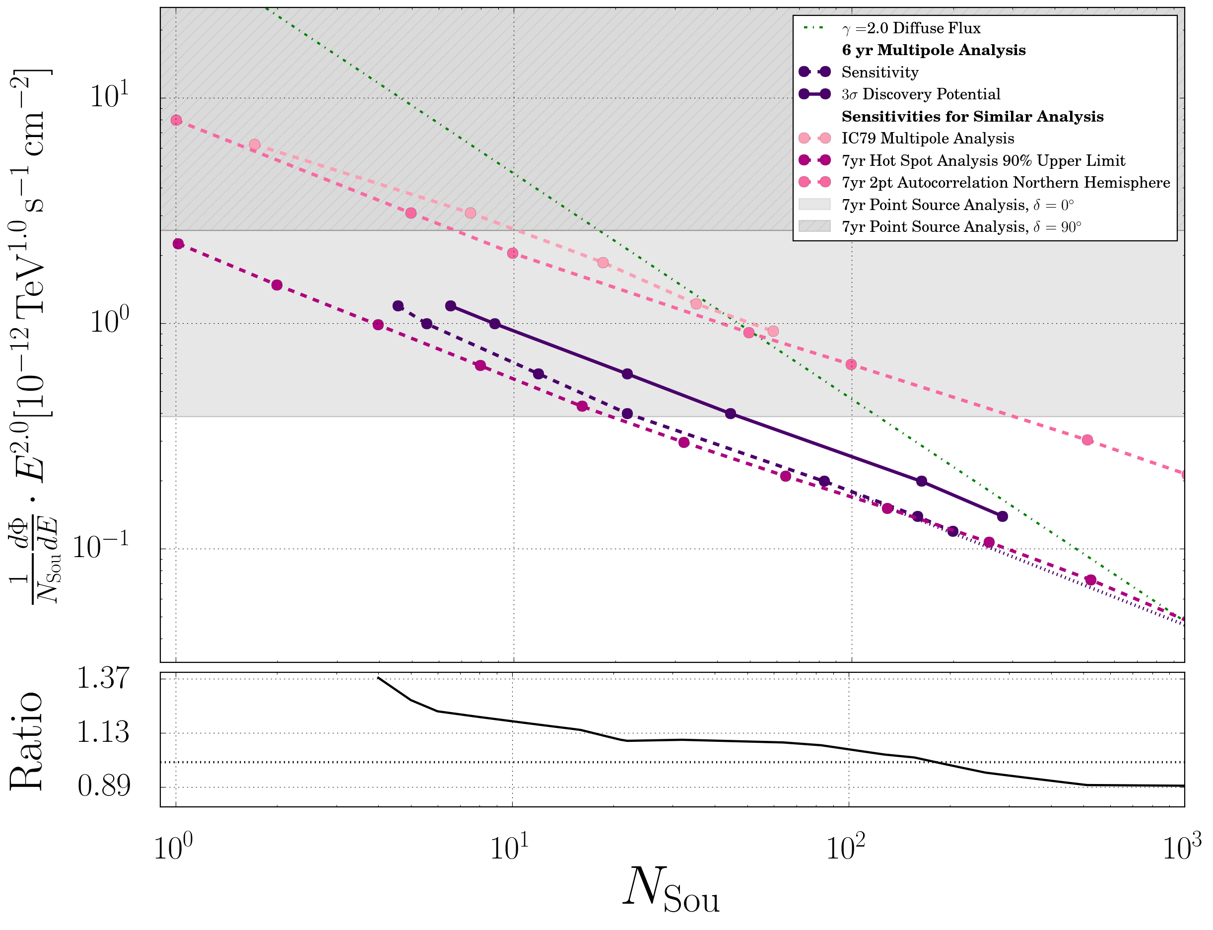
The \(\gamma=2.0\) plot is used to compare this analysis to other comparable ones. This implies that the plot also shows the results from the standard point source analysis and the previous IC79 Multipole analysis. The time developement of the multipole analysis can be read off from the senstivity lines and is approximately \(\Phi_{0}/N_{Sou}(t)\propto 1/t^{0.8}\) which is in good agreement with the time devolement of the standart point source analysis where \(\Phi_{0}/N_{Sou}(t)\propto 1/t^{0.7}\). As expected the point source search is more sensitiv for small number of sources whereas this analysis can be used for the case of many sources. A rough esimate of the maximum number of sources that this analysis is sensitiv to can be drawn from the crossing point of the sensitivity line with the Best-Fit Flux per Source from the diffuse fit. The value is estimated to be in order of \(10^3\). However, this estimation is based on the simulation of skymaps with a fixed source strength \(\mu\) only and therefore has only limited accuracy. A way of dealing with mixed skymaps using the given results is explained in section Possible Extensions

Fig. 23 Comparison of sensitivities from different analysis methods given in flux normalisation per source (\(\gamma=2.0\)). The plot at the bottom shows the ratio of this analysis’ sensitivitiy and the 7yr hot spot analysis’ 90% upper limit.

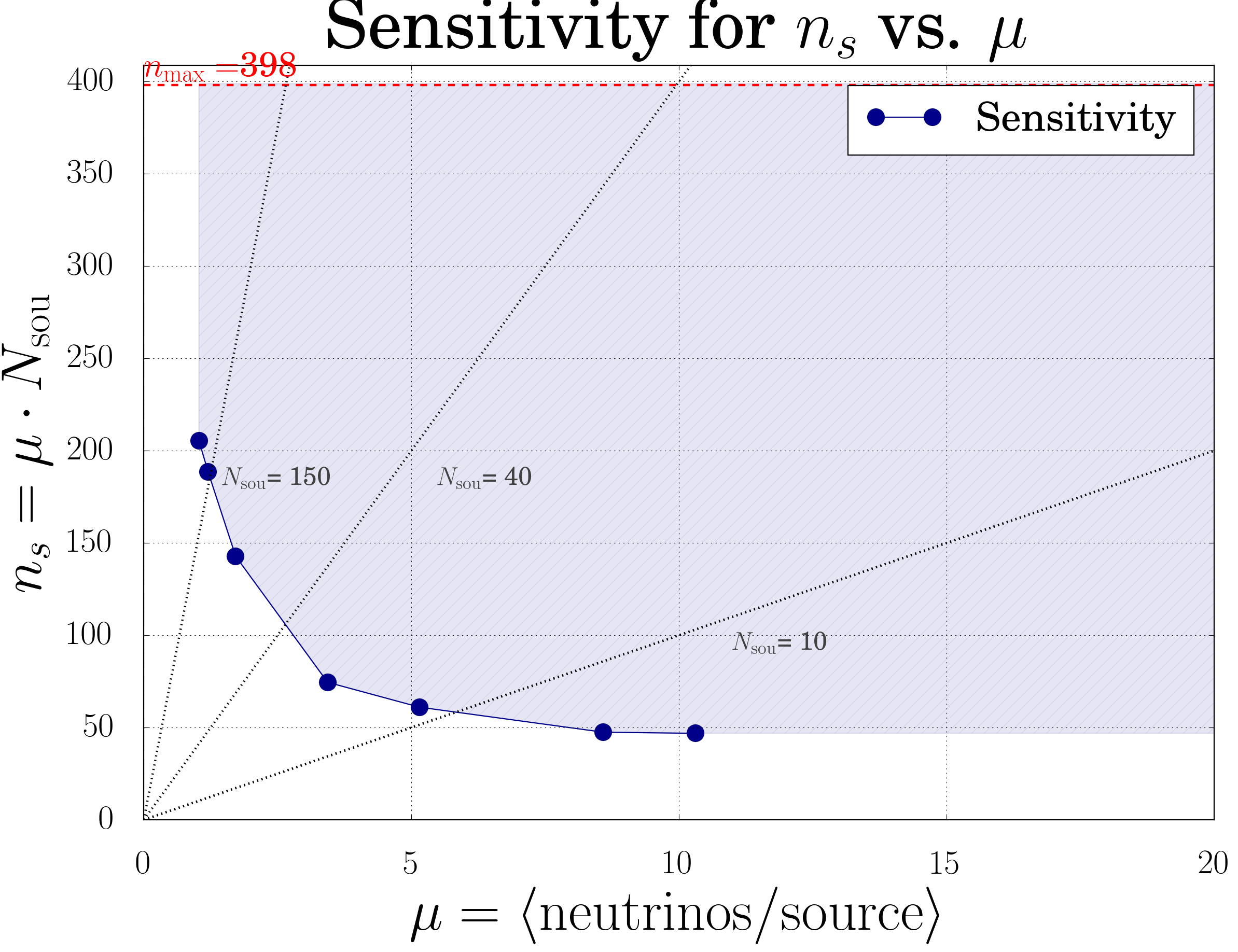
Fig. 24 Sensitiv parameter space of this analysis (\(\gamma=2.0\))

• \(\gamma=2.13\) (Best Fit)

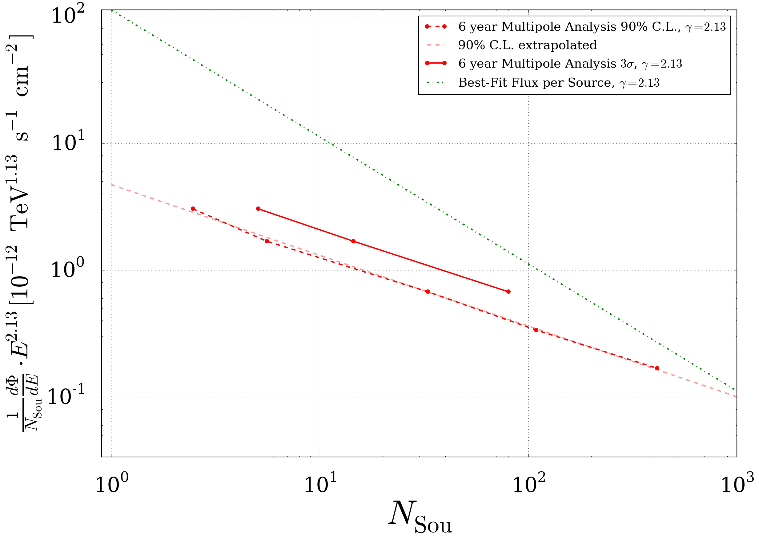
Fig. 25 Comparison of sensitivities from different analysis methods given in flux normalisation per source (\(\gamma=2.13\))

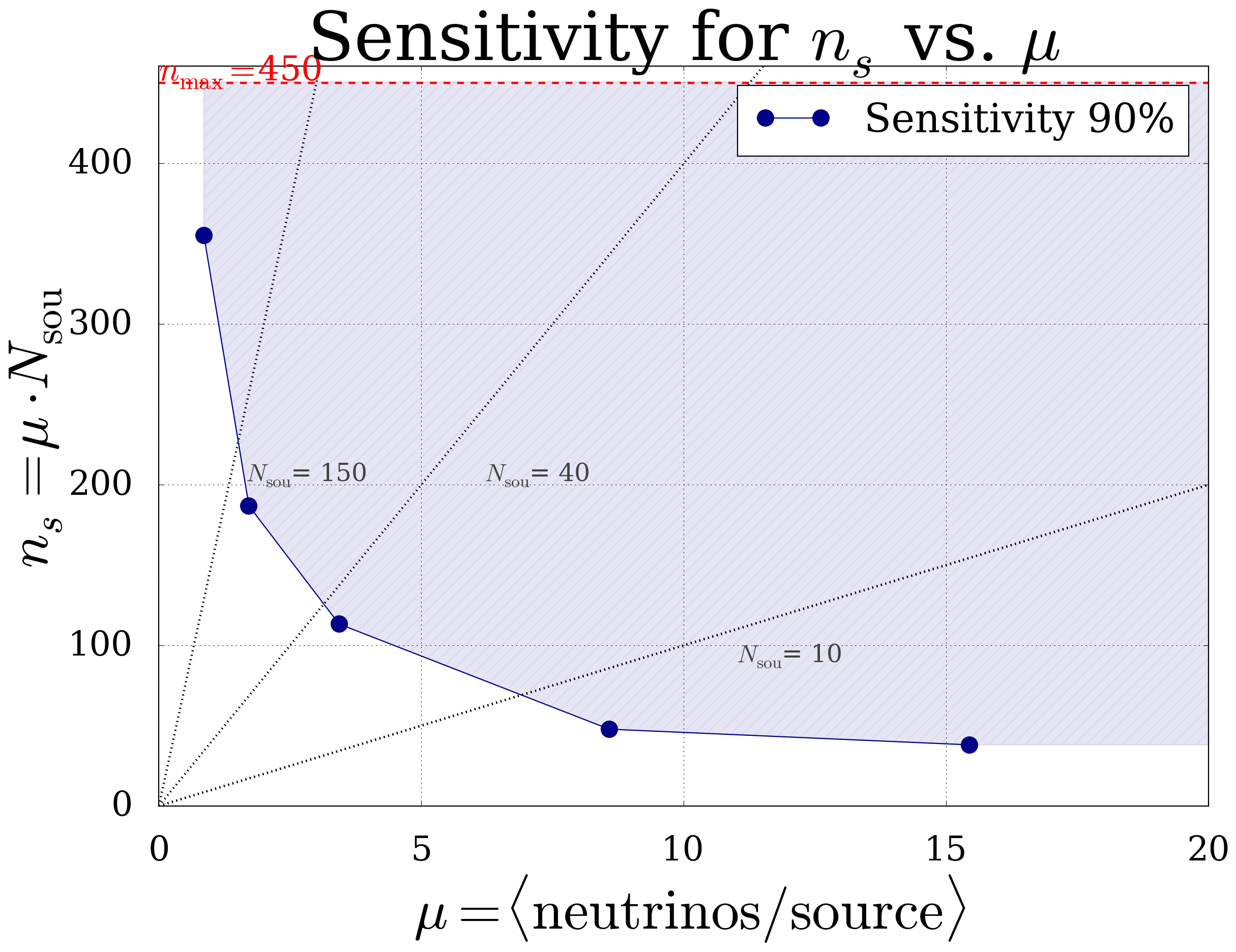
Fig. 26 Sensitiv parameter space of this analysis (\(\gamma=2.13\))