Post-unblinding Checks - reduction of zenith range to 90°-110°
Motivation of strict zenith cut
The unfolded ratios for September to November do not match in strength with the MCEq prediction based on the MSIS atmospheric model. Investigating the neutrino rate per month also indicate that the raise increase faster than decrease in fall. This is possibly related to the fast heating of the stratosphere in spring at the atmosphere around Antarctica. This process is related to pressure waves causing this so-called Sudden Stratospheric Warming.
The European Centre for Medium-Range Weather Forecasts (ECMWF) collects temperature data of the stratosphere measured on hourly basis from multiple experiments. The stratosphere consists of various pressure levels which each have their own temperature profile. More information about the layers and corresponding muon (also relevant for neutrino production) can be found in this paper. The zenith range from 90°-120° corresponds to latitudes from 90°S to 30°S. an illustration of these locations across the sky will be uploaded soon. The following plots depict the temperature profiles for various pressure levels relevant for neutrino production (dashed lines). The profiles are compared to the monthly neutrino rate within the zenith range from 90°-110° (for explanation why this range is regarded see below).
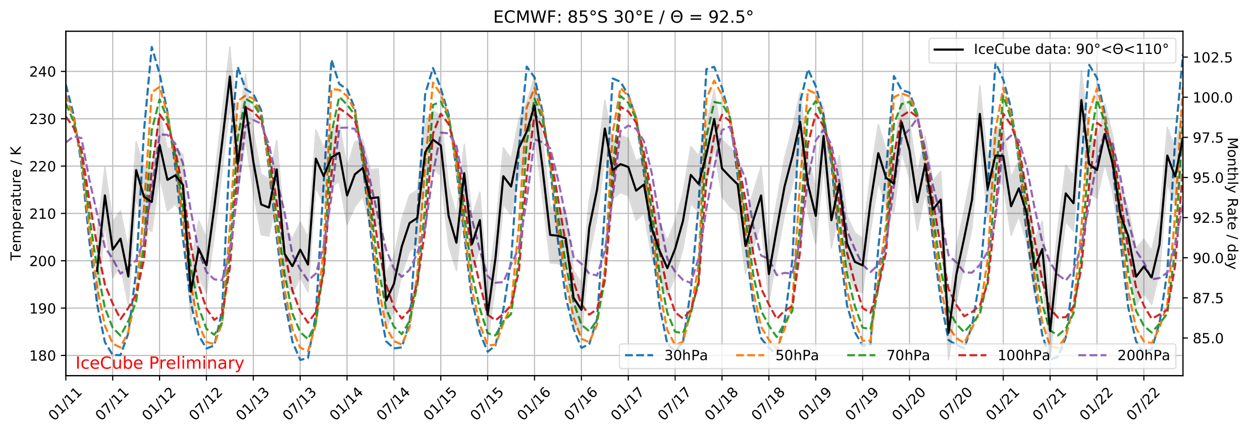
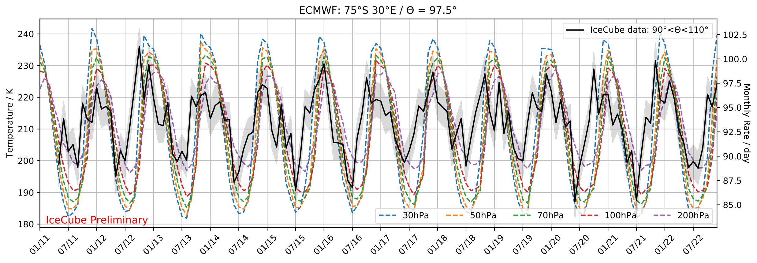
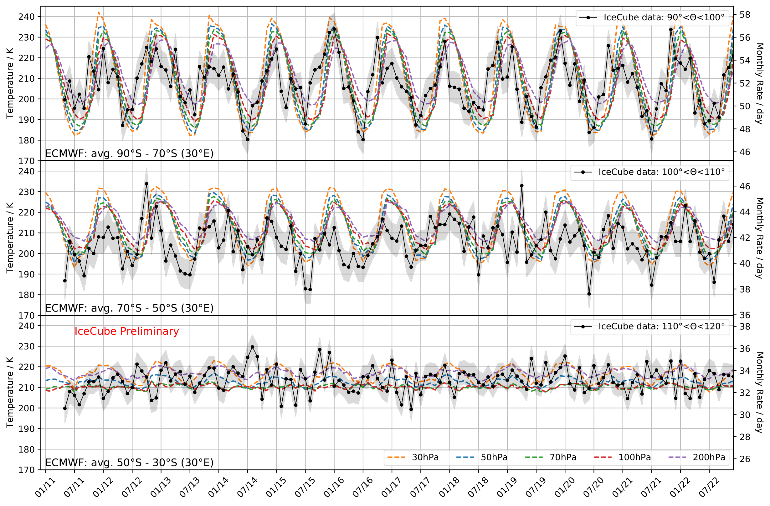
The temperature profiles are in phase with the neutrino data up to latitudes of 50°S (zenith: 110°). Whereas the temperature profiles are still in phase with the rates at 30hPa at 40°S, the pressure layers at 70hPa and 100hPa show are in opposite phase to the neutrino rate. This effect is even stronger at 30°S. All displayed layers are relevant for neutrino production and the opposite phasal behavior can impact the seasonal variation result. Especially the inverted pressure levels are contributing to the particle production. Production profiles versus slant depth are displayed here. The same profile will be obtained for neutrinos with MCEq. Cutting at the zenith region at 110° would yield an observation of larger variations, as can be observed in MCEq predicted ratios here.
The average monthly rate for zenith between 90°-110° is depicted below.
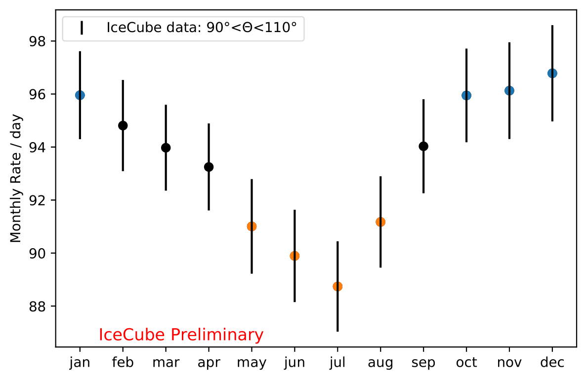
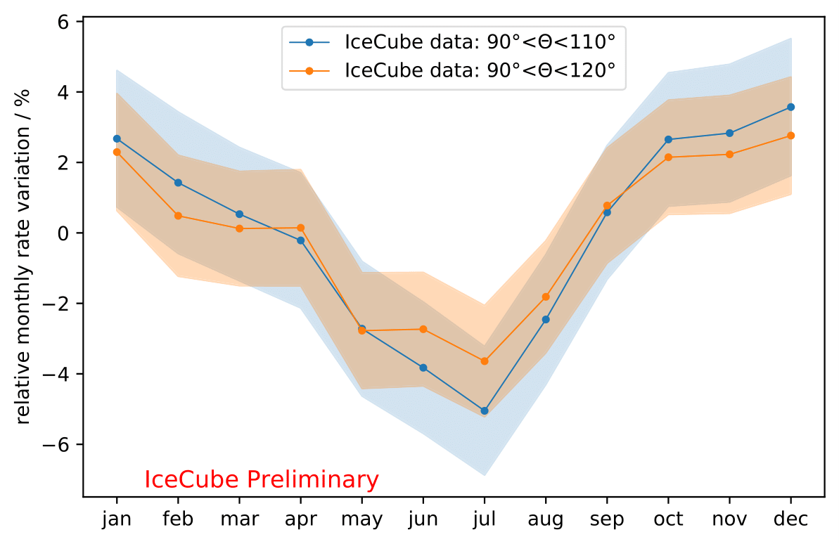
The rate variation is not symmetric across the year. The cooling (corresponding to rate decrease) is longer than the sudden increase in rate starting in August. In contrast to the split in austral summer and winter (jun-aug vs. dec-feb) as investigated by Honda et al., a new split into seasons based in similar rates is proposed: may-aug vs. oct-jan. This ensures that the variations can be measured at its most extreme times in the year.
Reducing the data set to zenith angles between 90°-110° only cases a loss of 26% of events. The systematic uncertainty is recalculated for the updated range. Studies on MC whether the unfold algorithm needs to be reoptimized is depicted in the sections below.
Unfolding of updated zenith range:
MC study
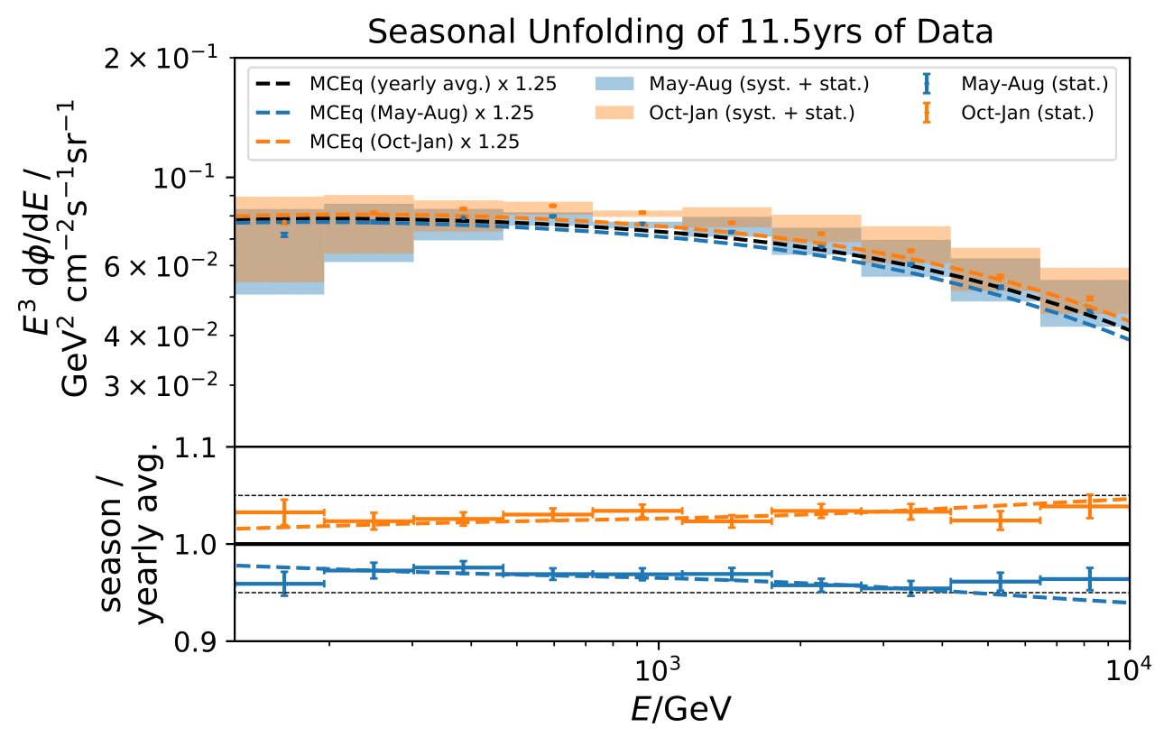
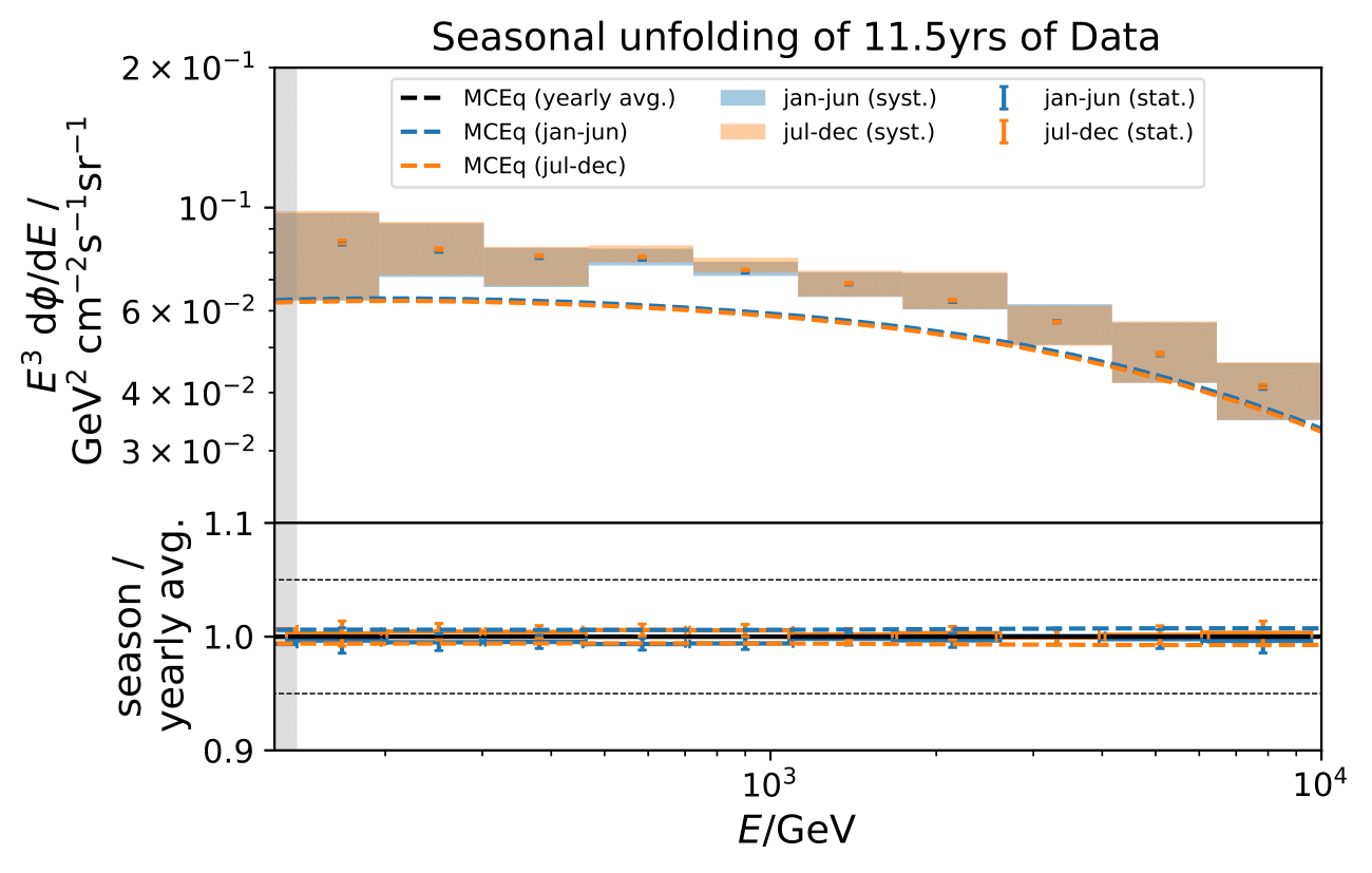
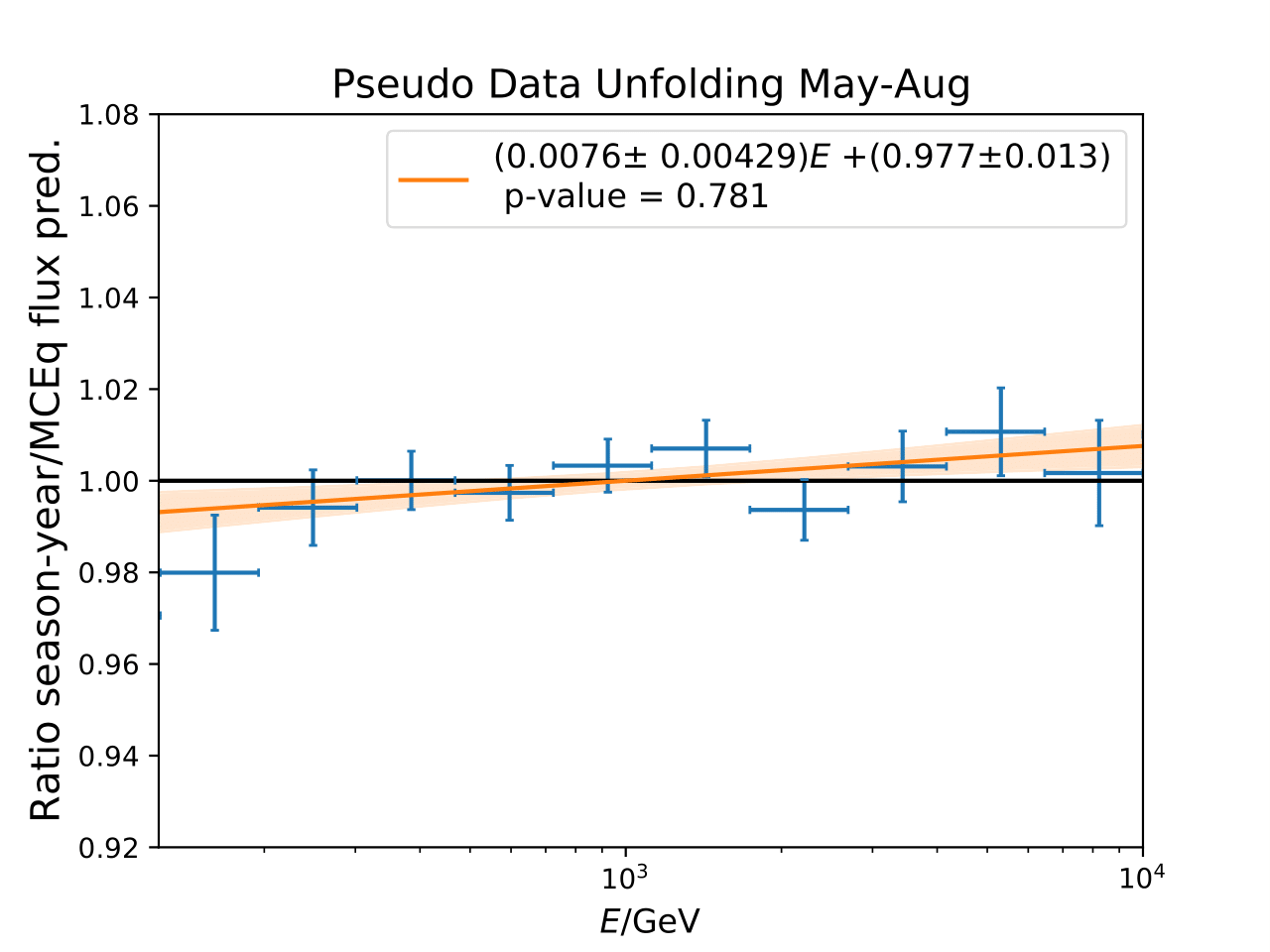
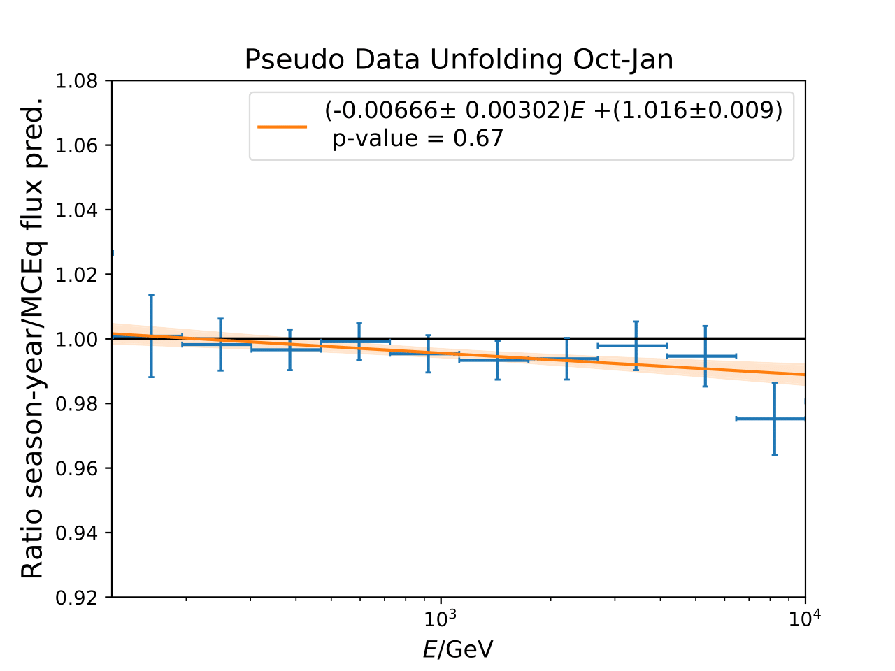
The feasibility of cutting the maximum zenith angle at 110° is evaluated on MC. Seasonal pseudo-data sets are generated from MCEq weights and unfolded. Theplot shows unfolding with the algorithm trained as it was, for the zenth range of 90°-120°.
The unfolded results are compatible with the prediction for both seasons.
The comparison between unfolded ratio and MCEq prediction is evaluated as a \(\chi^2\) goodness of fit as it was done previously. The hypothesis to be rejected is the compatibility of the unfolded ratio with MCEq. The hypothesis cannot be rejected for both seasons, which indicates that the seasonal unfolding is feasible without re-training DSEA.
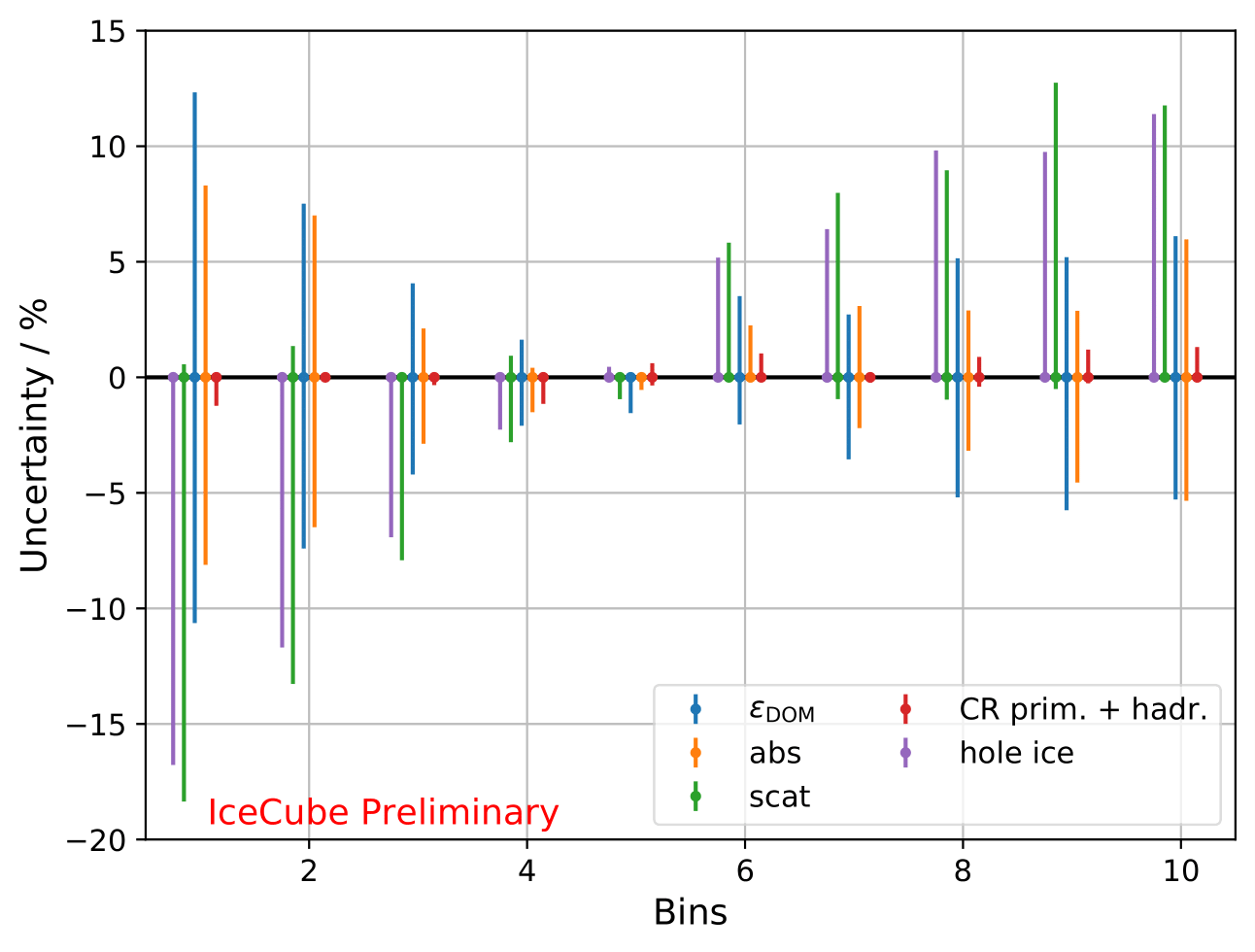
Systematic uncertainty
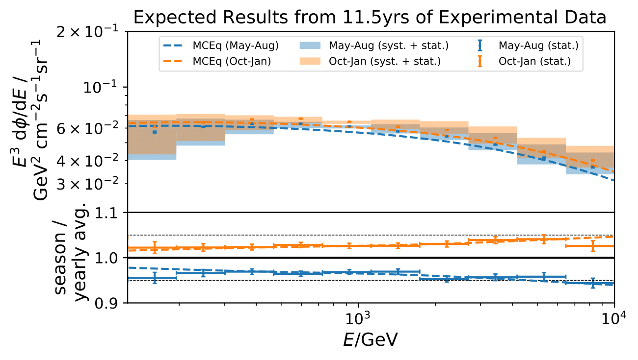
Calculated systematic uncertainties based on the cutted MC sample for 90°-110°:
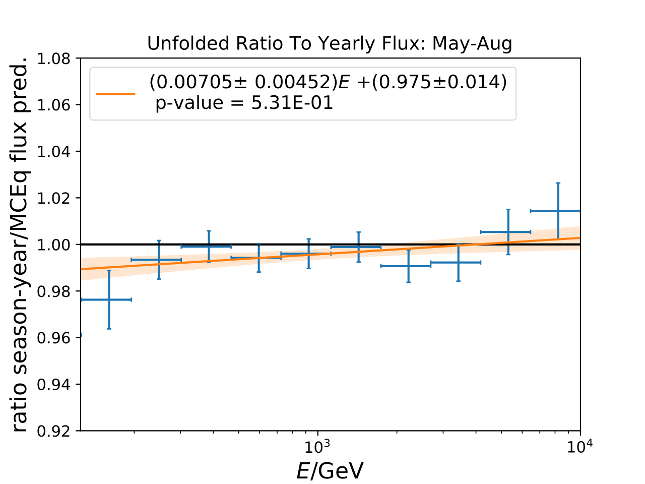
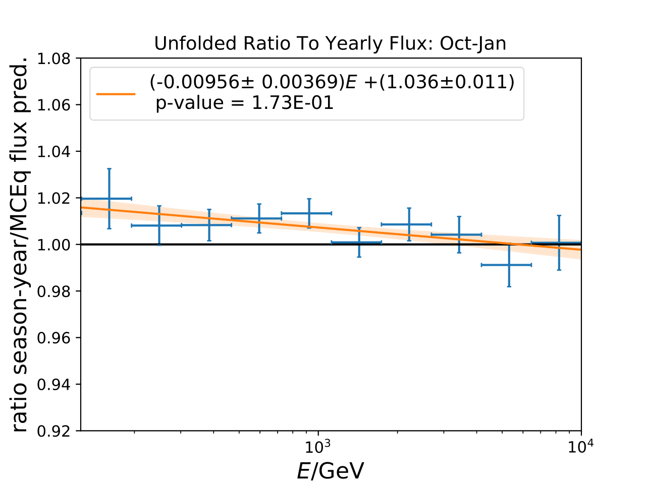
Compatibility to MCEq
Another \(\chi^2\)-test is performed to test the MCEq seasonal variation hypothesis. The seasonal variation predicted by MCEq is governed by the atmospheric model NRLMSISE-00. The corresponding tests and p-values are shown below. The hyothesis cannot be rejected for both austral summer and winter.
Season |
p-value (MCEq) |
\(\sigma\) variation |
|---|---|---|
may-aug |
\(5.31\times 10^{-1}\) |
13.2 |
oct-jan |
\(1.73\times 10^{-1}\) |
10.6 |