Unfolding

The energy of the neutrino cannot be measured directly. When a muon neutrino enters the ice, it undergoes a CC interaction: \(\nu_{\mu} +N \rightarrow \mu + X\). The observed rate of the neutrino induced muon depends on the neutrino spectrum convoluted with the probability that a muon neutrino propagates through the detector while producing a muon in the detectable energy range of IceCube:

\[\frac{\mathrm{d}N_{\mu}}{\mathrm{d}E_{\mu}} = \int_{E_{\mu}}^{\infty} \mathrm{d} E_{\mu} \left( \frac{\mathrm{d}N_{\nu}}{\mathrm{d}E_{\nu}}\right) \left(\frac{\mathrm{d}P(E_{\nu})}{\mathrm{d}E_{\mu}} \right).\]

The production and propagation of the muon are exposed to stochastic energy losses. This introduces a smearing on the solution as the muon energy, and hence the neutrino energy, cannot be determined directly. The reconstruction of the neutrino energy can be regarded as an inverse problem in unfolding, or deconvolution. The true energy distribution \(f\) of the neutrino has to be inferred from measured / reconstructed quantities, denoted as \(g\):

\[g(y) = \int A(x,y)f(x) \mathrm{dx}\]

Due to the limited amount of data, the inverse problem is transferred into an discrete equation:

\[\vec{g}(y) = \textbf{A}(E_{\nu},y)\vec{f}(E_{\nu})\]

The response matrix \(\textbf{A}\) corrects for bin-to-bin correlations and smearing effects within the detection process. These can be caused for instance by stochastic energy losses along the muon track inside the ice.

DSEA - The Dortmund Spectrum Estimation Algorithm

DSEA treats the spectrum reconstruction as a multinomial classification task in machine learning. The discrete energy binning that has to be set beforehand, is regarded as categories to classify events into.

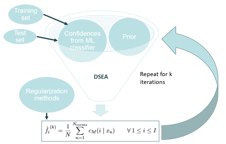
Illustration of the DSEA unfolding algorithm.

Any classification algorithm implemented in the sklearn python library can be selected as an input for DSEA. The training set is based on MC features which are found to be suitable estimators for the neutrino energy. The variable selection is explained in the next section. Confidences, some kind of probability estimates, predicted by the classifier are determined for each single event and given as an input to DSEA. These confidences are accumulated for each energy bin. This gives the overall probability of any event being categorized into a certain energy bin. If a prior pdf is given as an additional input, the classifier’s confidences are weighted by the prior pdf. If no prior is specified, a uniform distribution is set by default. The estimate \(f\) can be scaled by various regularization methods. Another possibility to regularize is the iterative application of DSEA. The estimate of the current iteration acts as the prior for the next one. However, the regularization parameters have to be chosen carefully. If the estimate is scaled too strongly, the optimum might not be found and the algorithm cannot converge. On the other hand, if the convergence is slowed down, the algorithm might not converge either.

Regularization Methods

The current estimate can be scaled by three step size decay functions. These functions allow to scale the prediction in each iteration in order to adjust the convergence speed. The current estimate is updated by:

\[\hat{f}^{(k),+} = \hat{f}^{(k-1)} + \alpha^{(k)} \cdot p^{(k)}\]

with the step size \(\alpha \geq 0\) (the scale factor of the convergence speed) and the search direction which is given by

\[p^{(k)} = \hat{f}^{(k)} - \hat{f}^{(k-1)}.\]

A step size of \(\alpha = 0\) corresponds to no regularization via step size decay. In this case the regularization is regulated via the number of DSEA iterations.

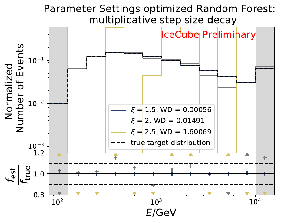
Multiplicative step size decay: \(\alpha_{\mathrm{K}} = k^{\xi -1}\).

Exponential step size decay: \(\alpha_{\mathrm{K}} = s \cdot\xi^{k -1}\) with a start size \(s\).

Adaptive step size decay: \(\alpha_{\mathrm{adaptive}} = \arg \min \limits_{\alpha^{(k)} \geq 0} \hat{l}_r^{(k)}(\hat{f}^{(k-1)} + \alpha^{(k)} )\)

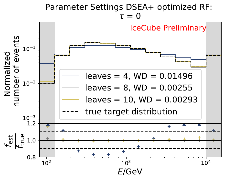
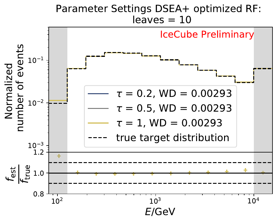
In addition to the previously shown methods, the adaptive step size decay adjusts the step size according to the previous estimation and the search direction. Hence, the step size does not remain constant in each iteration. While the other methods might not be able to find the optimal solution because the step size decay was chosen too widely, the adaptive approach allows to shrink the step size when the optimal solution is close. The function \(\hat{l}_r^{(k)}\) to minimize is the objective function given by the RUN algorithm. The step size is adapted to the current estimate maximizing the likelihood of the next estimate in the search direction. This procedure is similar to a line search in numerical optimization. The step size itself can be regularized by the regularization strength \(\tau\). If \(\tau=0\), the step size is unregularized and is only regulated via the flattening of the second derivative of the objective function.

The unfolding input must be discretized in order to calculate the adaptive step size. This is done by a decision tree. The maximum number of leaf nodes (referred to as \(l\)), which corresponds to the number of clusters in the multidimensional discretization of the input, can be adjusted by the user. Further description of the parameters can be found here and in the source code.

Parameter Optimization

To find the optimal parameters for unfolding with DSEA, initial unfolding variables have to be selected. These variables have to be well-correlated with the neutrino energy. The correlation between each variable to one another cannot be avoided since the reconstruction algorithms all rely for instance on the number of DOMs which detected photoelectrons within an event. A set of five initial unfolding variables is selected by considering previous unfolding analyses. An overview and description are shown in the table below. After the parameters are optimized, a further variable selection is performed using a coverage and bias test.

Description of Variables:

• n_doms (L5_nch, BestTrackDirectHitsICC.n_dir_doms,*HitMultiplicityValues.n_hit_doms*):

  Number of channels: DOMs detecting photoelectrons (P.E.) per event.
• n_pulses (BestTrackDirectHitsICC.n_dir_pulses) :

  Number of detected pulses based on direct hits from best reconstructed track.
• Q_tot (BestTrackDirectHitsICC.q_dir_pulses) [P.E.]:

  The total deposited charge inside the detector of the best reconstructed track based on direct hits. Measured in number of photoelectrons.
• EtrunDoms (SplineMPEICTruncatedEnergySPICEMie_BINS_Neutrino.energy) [GeV]

  Truncated neutrino energy: Energy estimator of the neutrino based on the energy loss of the induced muon. The track is binned in a discrete manner based on the track length.

  The ratio of the observed P.E. to the estimated P.E. with fixed energy loss is calculated for each bin. Bins with high energy losses are discarded and the mean is determined over the remaining bins. The Bins approach is analogous, but uses continuous bins of track segments along the muon path. Both algorithms lead to very similar results.
• l_track (BestTrackDirectHitsICC.dir_track_length) [m]:

  Track length of a muon: Projection of direct hits along a muon track within the time window C (-15ns < \(t\) < 75ns) determined for the best reconstructed track based on direct hits
• direct_hits (L5_ndir_c)

  Number of direct photons: unscattered photons by ice impurities within the time window C.

More information on the variable definitions can be found here, here, here and here.

A grid search over the complete parameter space would be computationally too expensive, considering that many different classifiers can be used, so that three settings are tested for each parameter. The unfolding result is obtained via 10-fold cross-validation. The MC set is divided into 10 equal parts. 9 out of 10 are selected for training DSEA whereas the remaining one acts as the test set. In the next step, another one out of the 10 sets is selected for testing and the remaining ones are used for training. This procedure is repeated until every set has been once selected as the test set. The prediction is then averaged over all ten iterations. The Wasserstein Distance measures the deviation between the MC truth and the estimation from DSEA. The number of DSEA iterations is set to 7 as all selected classifiers converge to an estimation after these number of iterations. Besides the classifier parameters, the regularization parameters have to be chosen carefully. There is a trade-off between an optimal solution keeping all features of a spectrum and the smoothing of the distribution.

The neutrino events are unfolded into ten logarithmic energy bins between 125.9 GeV to 10 TeV. An underflow and an overflow bin are defined below and above this energy range to account for the smearing into neighboring bins. No events below 100 GeV are present in the MC sample, however this could be the case in real data.

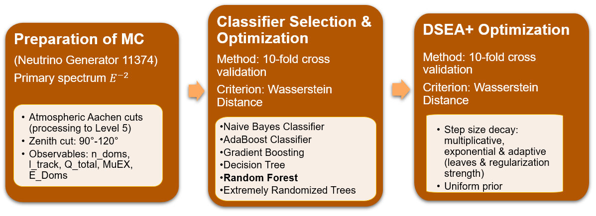
Optimization scheme of DSEA parameters.

Initial Optimization

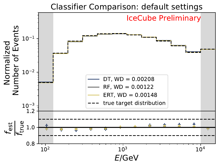
The parameter optimization on five energy-correlated variables on MC is displayed below. The MC generation spectrum is \(E^{-2}\). 500000 events are used for CV. The number of iteration is set to 7.

Six classifiers are tested within DSEA at their default settings:

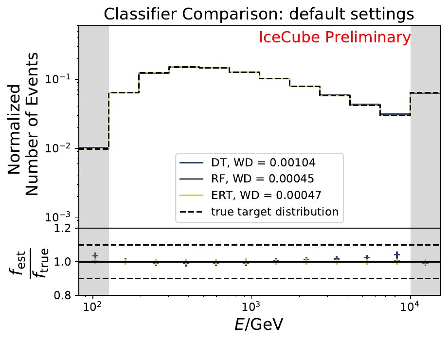
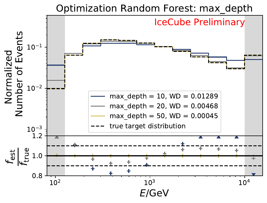
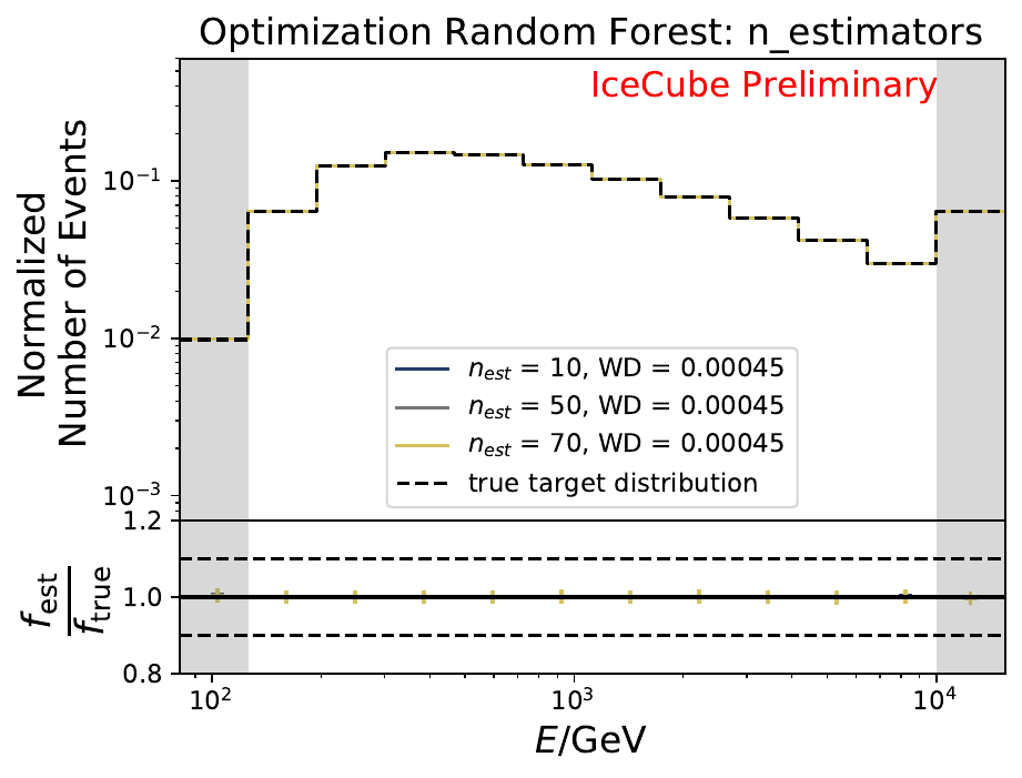
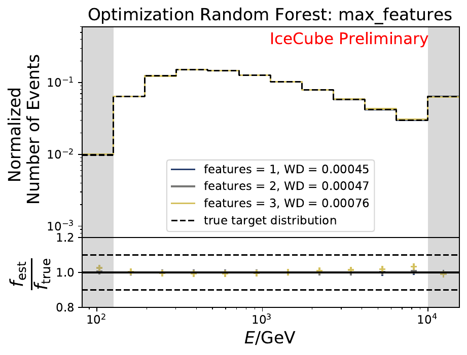
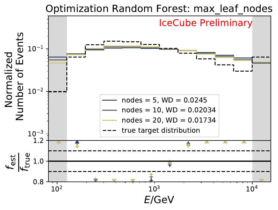
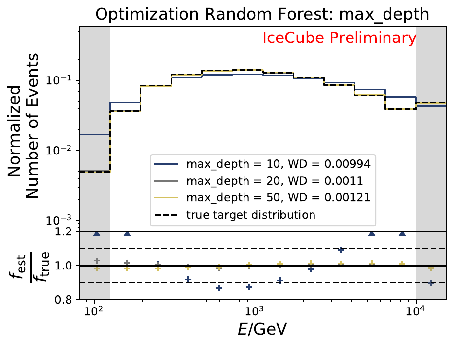
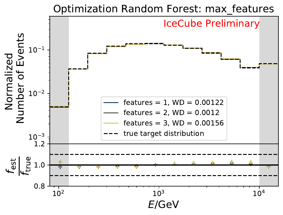
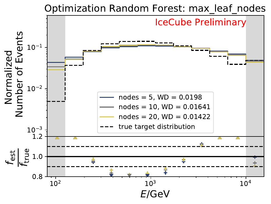
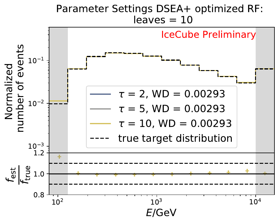
The best performing classifier (the Random Forest Classifier) is further investigated. To test if any Random Forest parameter does improve the unfolded result, four parameters are tested in detail. Since the Wasserstein Distance remains similar, and even increases for the maximum number of leaves nodes, the default Random Forest classifier is selected for unfolding at its default settings. These are shown in the table below. The following plots are not displayed here and will be updated shortly.

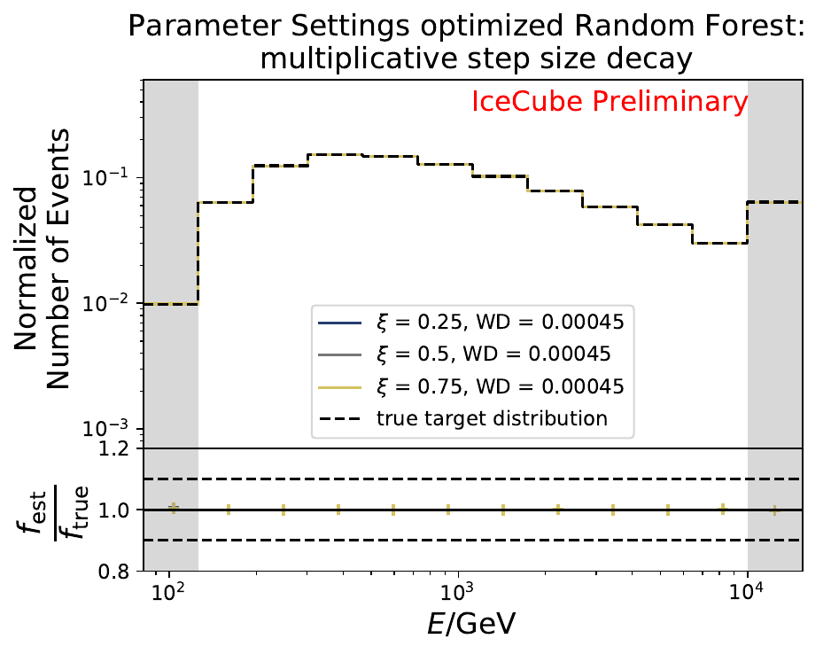
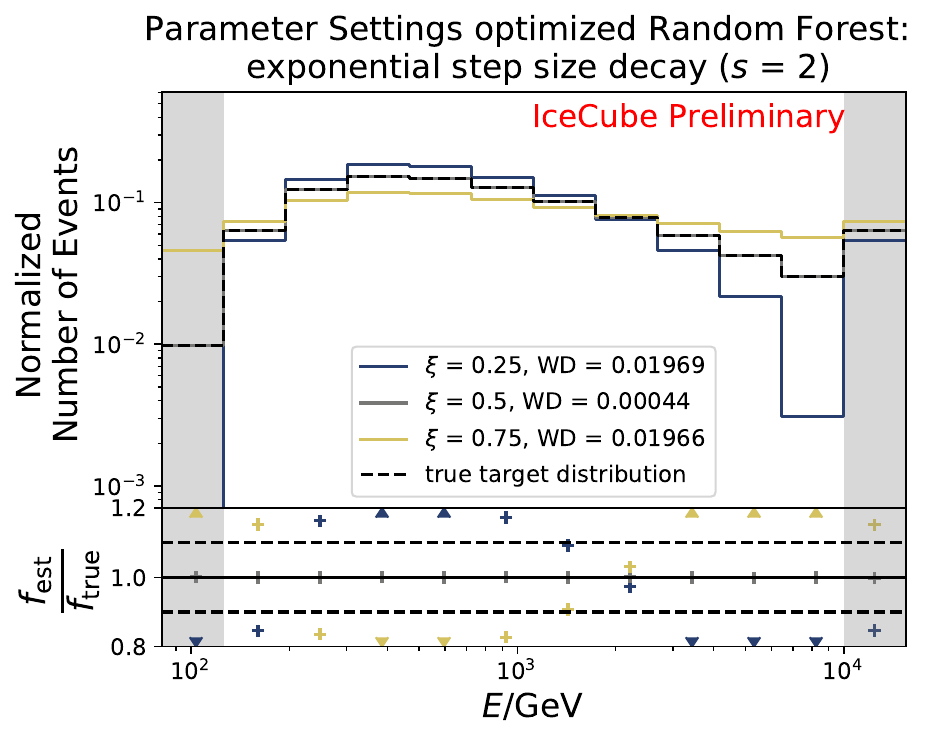
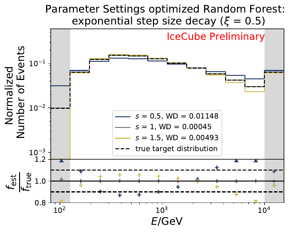
The smallest Wasserstein Distance of 0.00045 is obtained with the exponential step size decay method with a start size of \(s=1\) and a decay factor of \(\xi=0.5\). These settings are fixed for the following analysis.

Random Forest Default Settings

Parameter	Value	Definition
n_estimators	100	number of trees
max_features	\(\sqrt{N_{features}}\)	observables for best split
criterion	Gini-index	quality measure for split
max_depth	unlimited	maximum tree depth
min_samples_split	2	min number of samples to perform split
min_samples_leaf	1	min samples to create leaf node
min_weight_fraction_leaf	0	required sum of weights to create leaf node
max_leaf_nodes	unlimited	max number of leaf nodes
bootstrap	True	different random sub-set for each tree
min_impurity_decrease	0	decrease of Gini-Index to create split

Optimization on Atmospheric MC

Test of optimized parameters with best variables (from Variable Test Section) for original \(E^{-2}\) spectrum with all events (1.8 million)

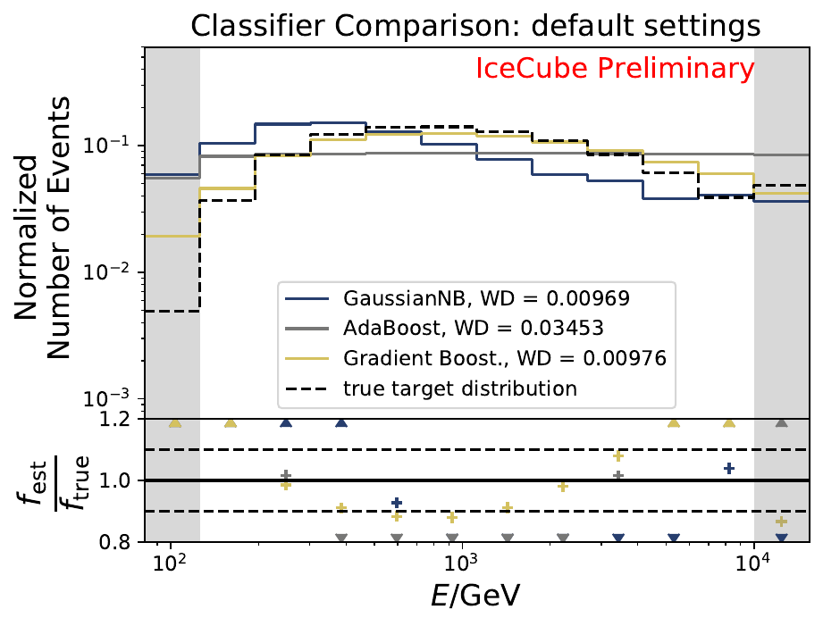
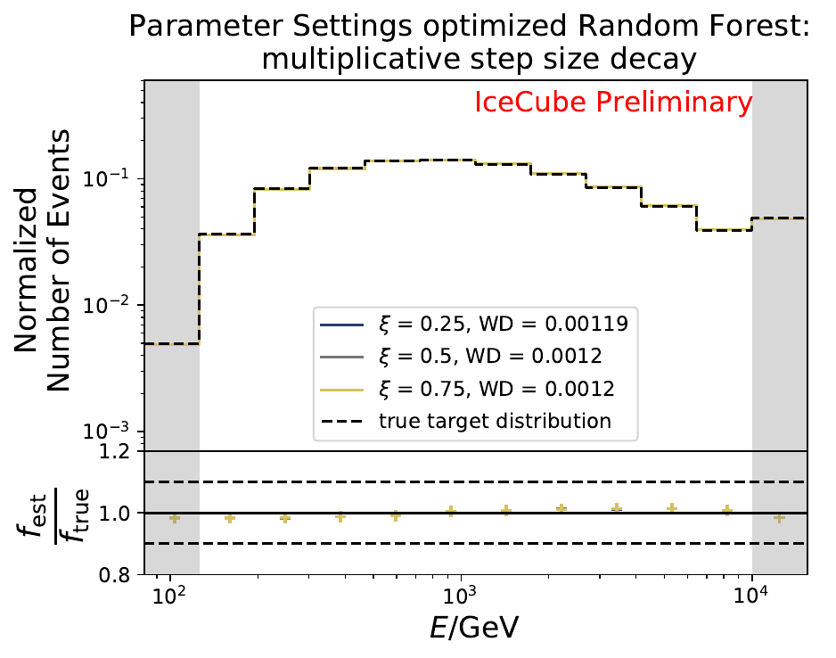
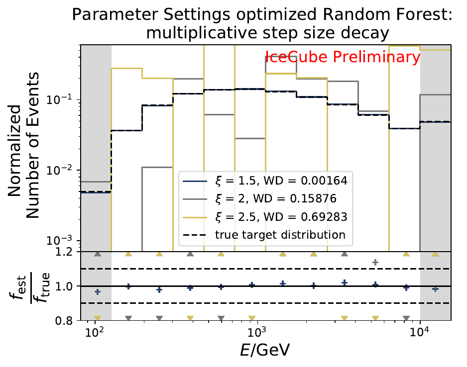
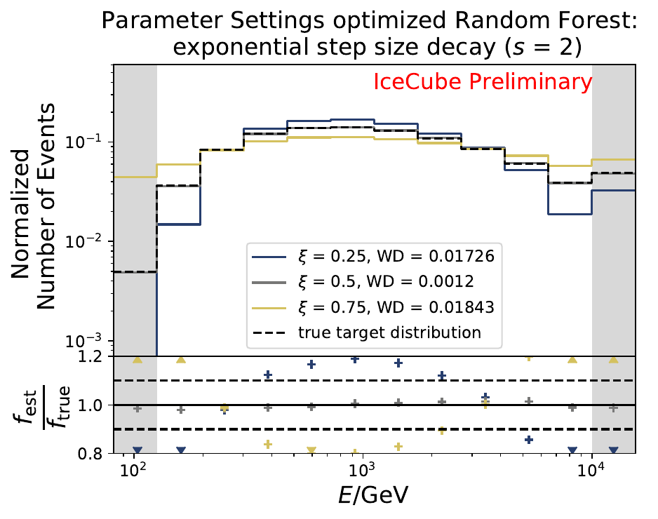
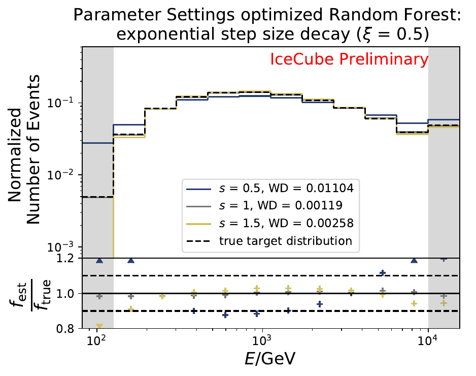
The smallest Wasserstein Distance of 0.00119 is obtained with the exponential step size decay method with a start size of \(s=1\) and a decay factor of \(\xi=0.5\). These settings are fixed for the following analysis. The optimization of the number of estimators in the random forest is not displayed above since the runtime increased tremendously for \(n_{\mathrm{est}}=70\). The previous optimization using all five variables showed that the variation of this parameter has only a small impact on the unfolded result. Not all classifiers have been evaluated again on this variable combination since the AdaBoostClassifier, the Gaussian Naive Bayes Classifier and Gradient Boosting Classifier were not suitable for this unfolding problem.

Variable Selection

After the optimal parameters are found, the selection of unfolding variables is investigated further. This can be done by investigating the coverage and the bias which is introduced on the unfolding result by the Monte Carlo simulation. These stability tests show that the combination of the five initially selected variables is not optimal. The combination of input variables is varied between two to five energy-related estimators. The one yielding the smallest bias and the best coverage is chosen as the final variable combination. Since the parameter optimization of DSEA is variable-dependent, the optimization procedure is rerun for the final variable choice.

The following tests are conducted in the same manner: The resampled atmospheric MC set (100 000 events) is divided to \(\frac{1}{3}\) corresponding to the test set and \(\frac{2}{3}\) as training sample in each of 2 000 iterations. DSEA is applied with the optimized parameters and the resulting pdf is scaled to the total number of events per bin. The coverage and bias values are calculated per energy bin and the distributions are displayed below.

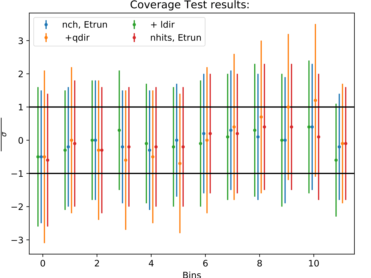
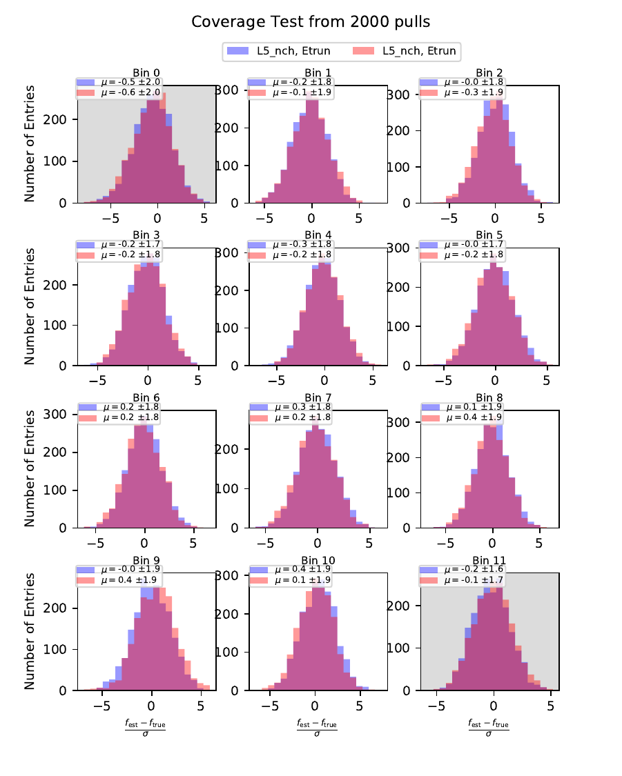
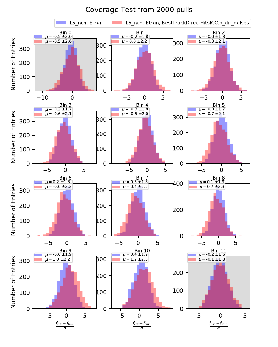
Coverage Test

The coverage test determined how well the unfolded result is covered within statistical uncertainties. This helps to determine if uncertainties are overestimated or underestimated. The coverage is defined as follows:

\[c_i = \text{coverage}_i = \frac{f_{\mathrm{est},i}-f_{\mathrm{true},i}}{\sigma_i}.\]

The deviation of the unfolded number of events to the MC truth per bin should not exceed one standard deviation. If this is the case, the variable selection introduces some additional uncertainties on the result. If the deviation lies well within one standard deviation, the statistical uncertainty is underestimated and works as a conservative measure. The standard deviation is obtained from the Poisson statistics: \(\sigma_i = \left(\sum_j \sqrt{\text{weights}_j}^2\right)\).

The event weights can be obtained within DSEA from the classifier outputs. This is one advantage of DSEA compared to other unfolding algorithms where only the unfolded spectrum is returned but information about each event do not remain accessible.

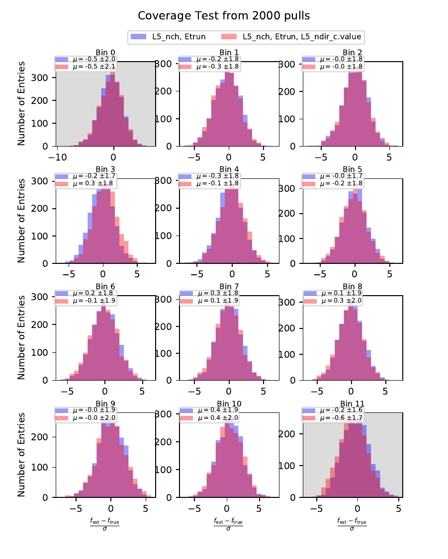
orange: nhit, truncated energy

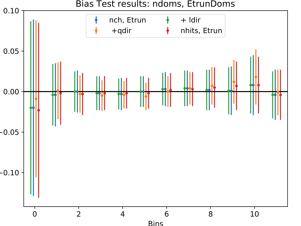
Bias Test

The bias test determines whether the variable selection introduces some additional bias on the unfolded event spectrum. It determines the relative deviation from the MC truth:

\[b_i = \text{bias}_i = \frac{f_{\mathrm{est},i}-f_{\mathrm{true},i}}{f_{\mathrm{true},i}}\]

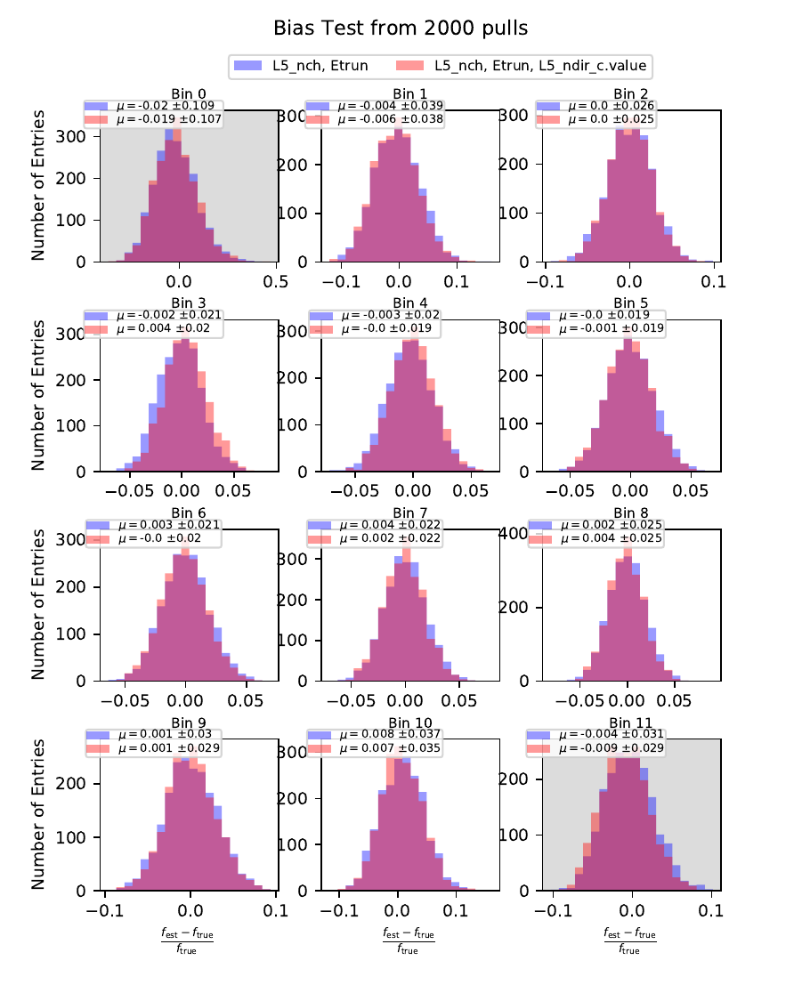
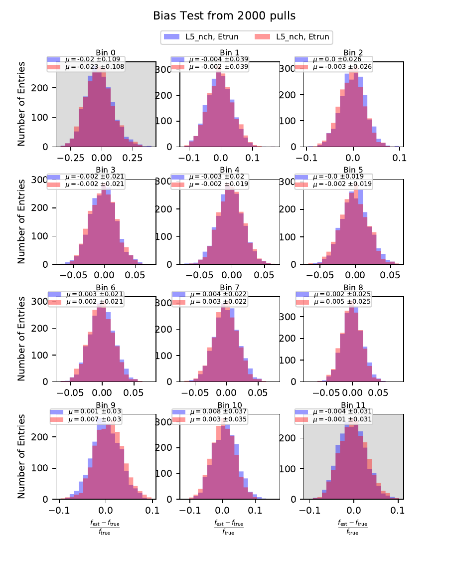
Test Results

Comparing the bias and coverage test results per each bin, the optimal variable selection is determined by choosing the combination with the smallest coverage and bias values. The same variables are tested as displayed in the section on Pass1. As could be expected from pass1 optimization, L5_ndir_c can be discarded. The combination of the truncated energy estimator and number of channels yields the most stable result. Unfolding based on one variable has the risk of being highly dependent on one single variable.

The bias and coverage test results are summarized below.