Expected Results / Burnsample Unfolding

Flux Normalization

To obtain a particle flux, the number of events per bin is divided by the energy bin width, the solid angle and the effective area:

\[\phi_i = \frac{N_i}{\Delta E \cdot A_{\mathrm{eff}} \cdot t \cdot (\cos(\Theta_{\mathrm{min}}) - \cos(\Theta_{\mathrm{max}}))}\]

The effective area describes the area of a 100% efficient detector which has the same event selection and trigger. It allows to normalize particle fluxes so that the results from different experiments become comparable. The documentation of how to calculate an effective area for neutrino-generator simulations can be found here. The effective area is calculated per energy bin using the simulated events from the training sample. Since the effective detection area is strongly zenith-dependent, the area is calculated for the zenith range from 90°-120° in four equidistant bins in \(cos(\Theta)\).

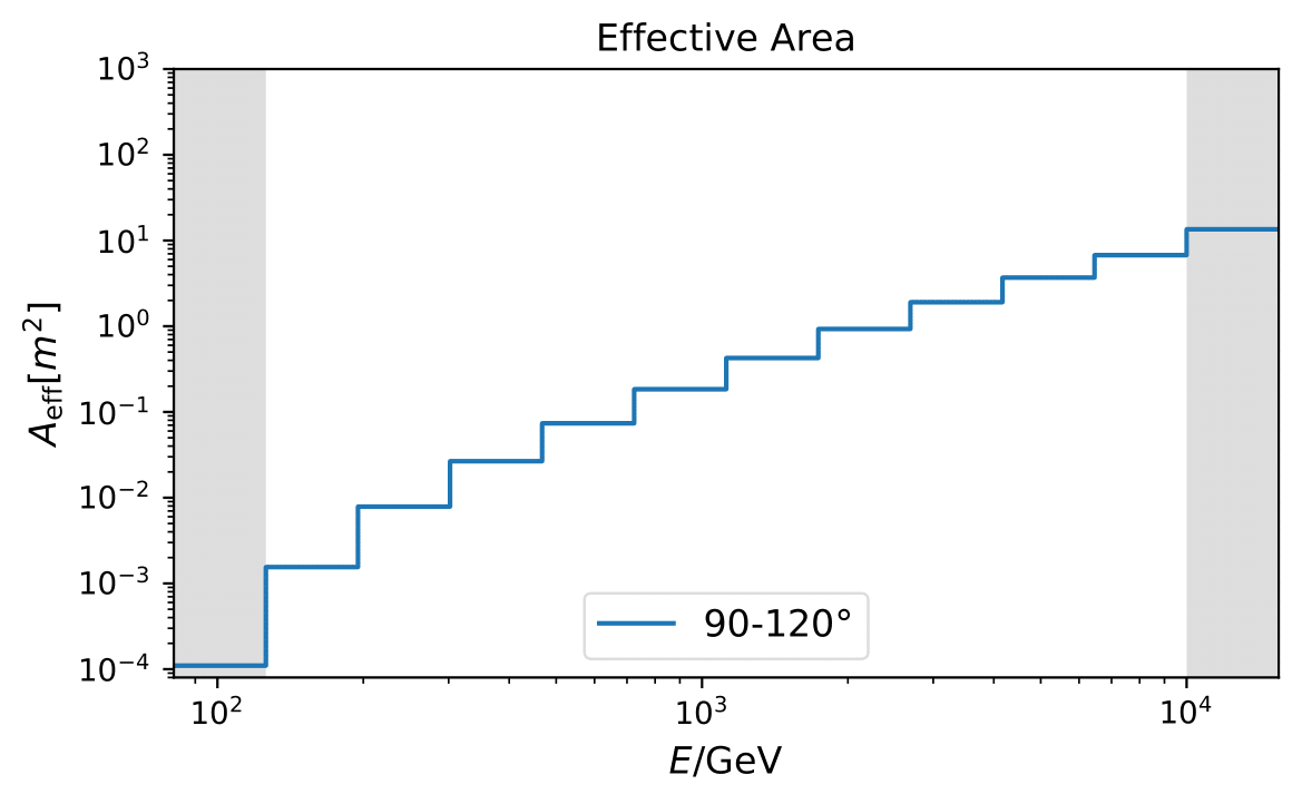
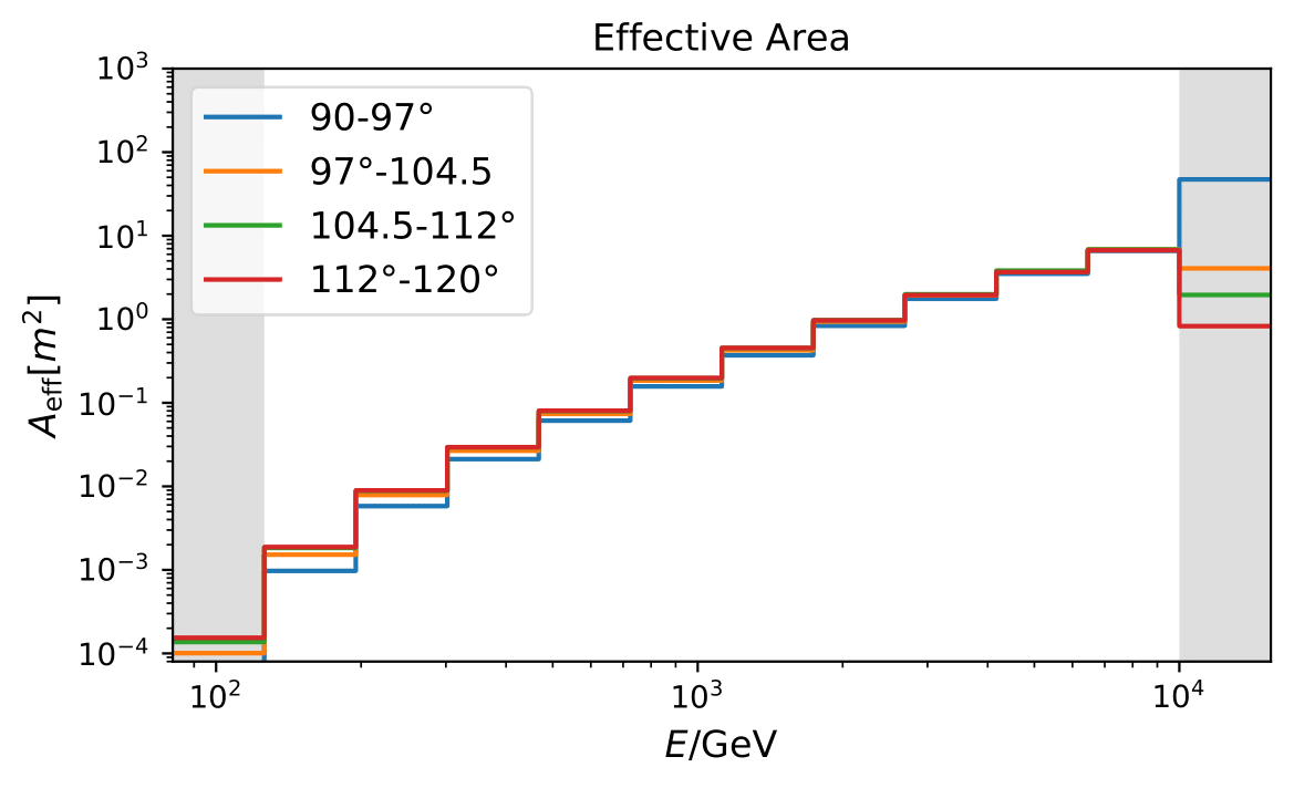
The effective area is obtained from simulation given finallevel processing of the Aachen sample. Any sources of uncertainties in the simulation are not considered as of now.

Unfolding Results from Burn Sample

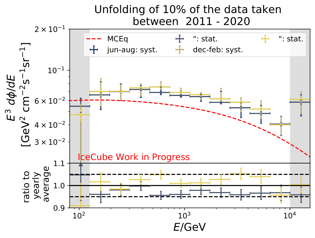
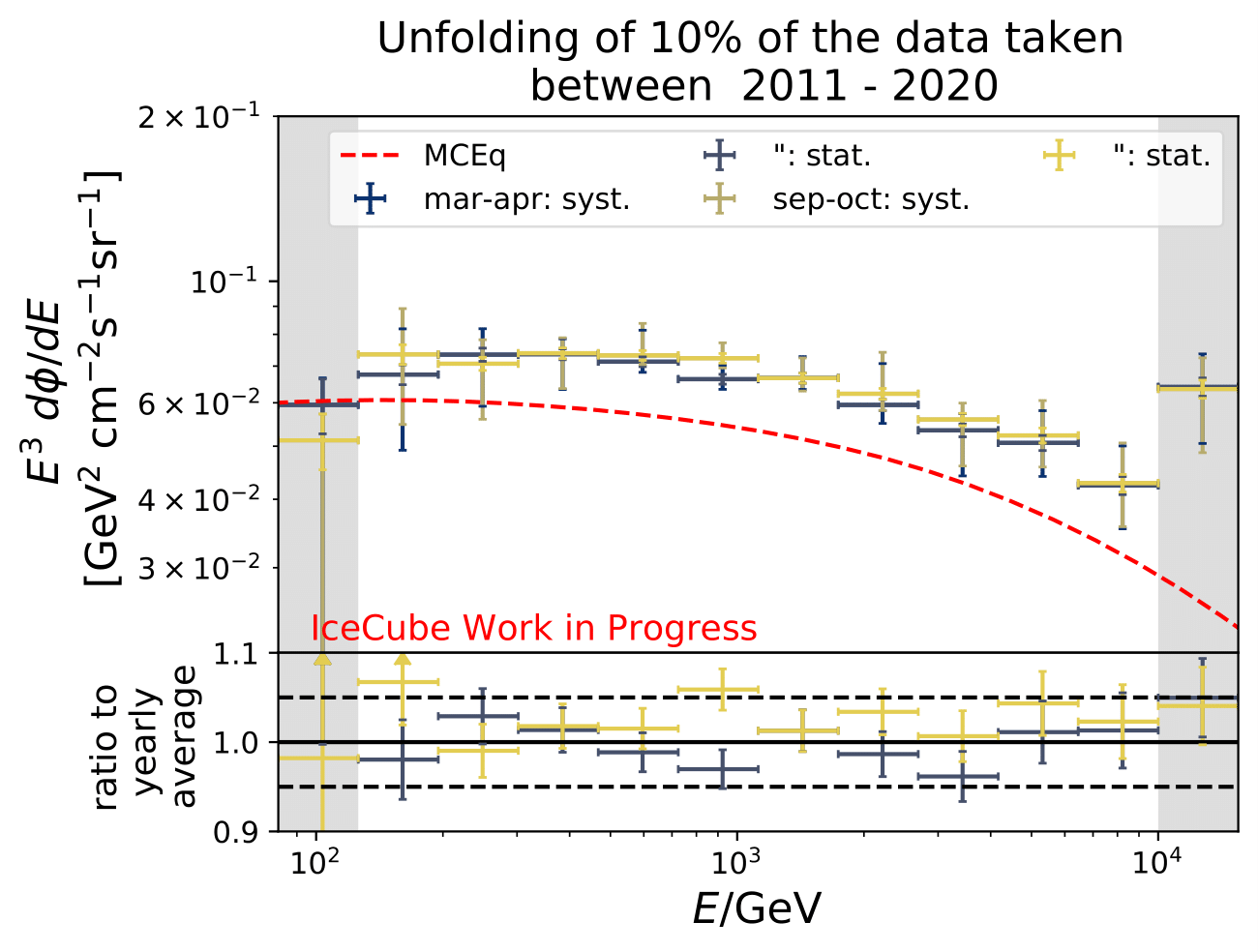
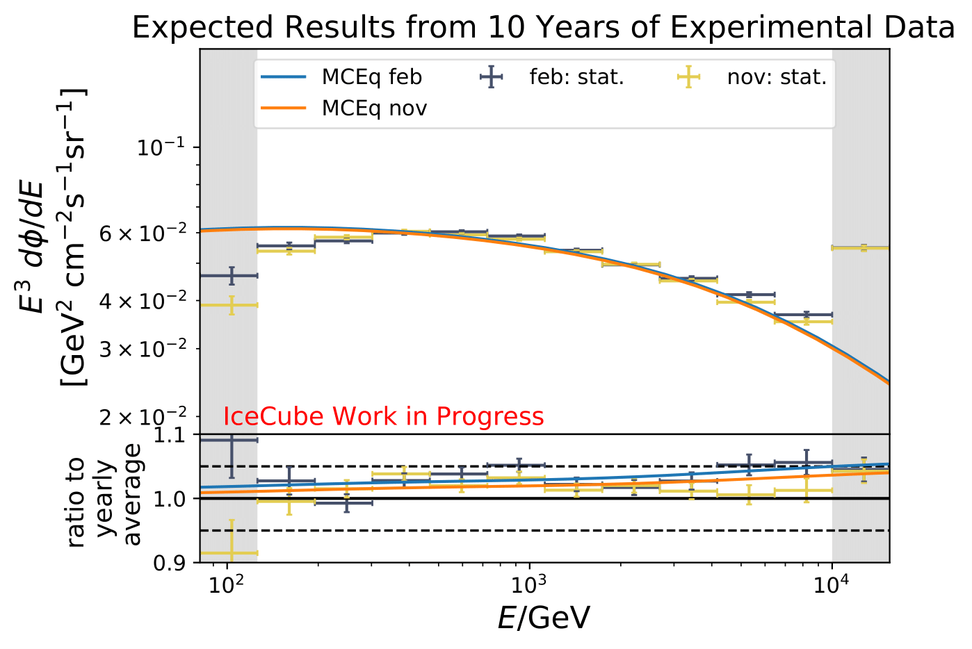
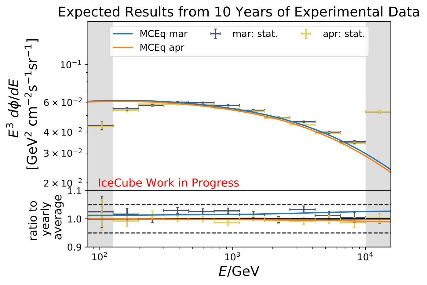
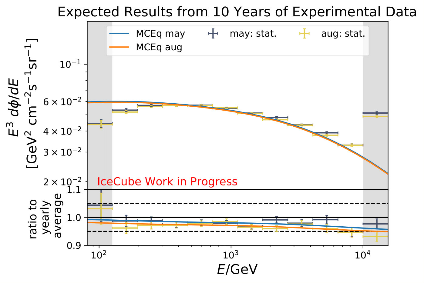
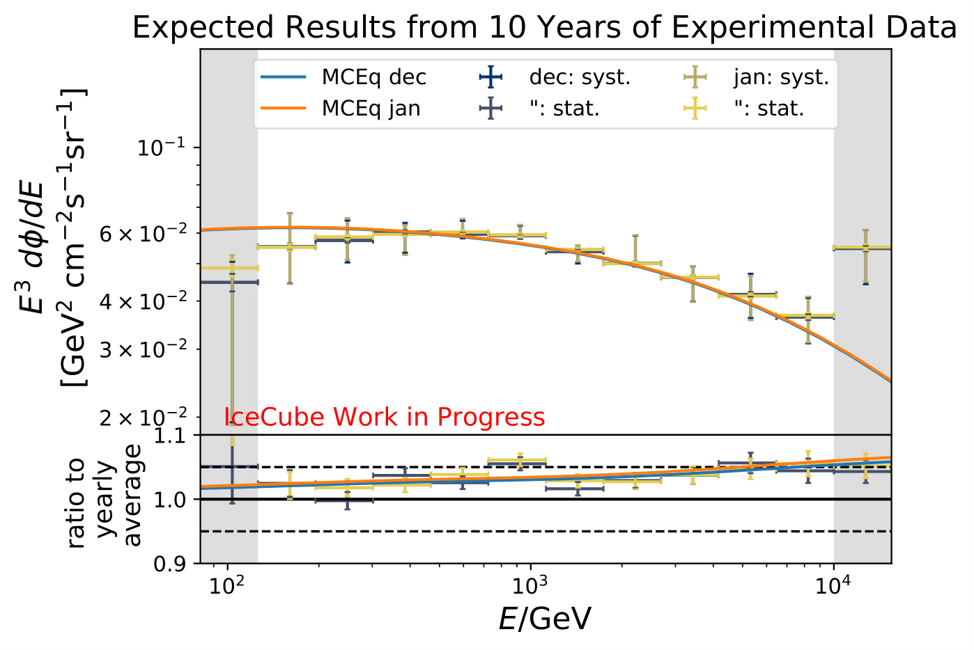
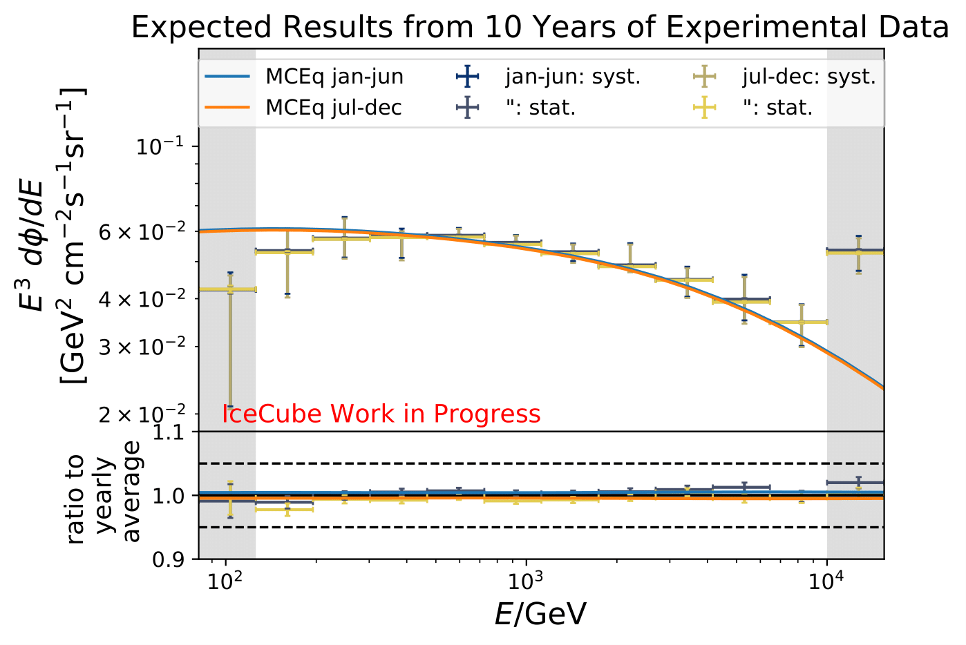
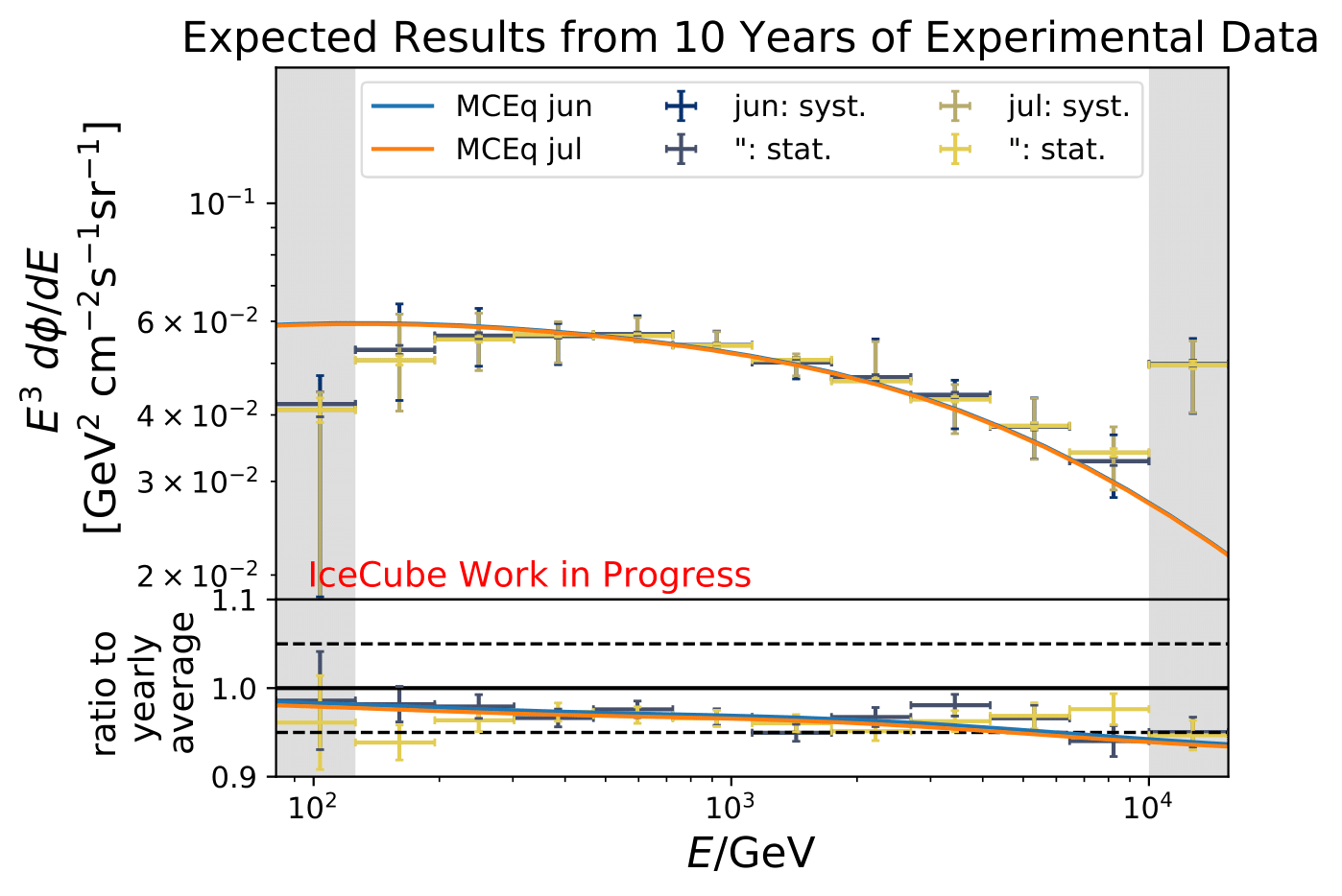
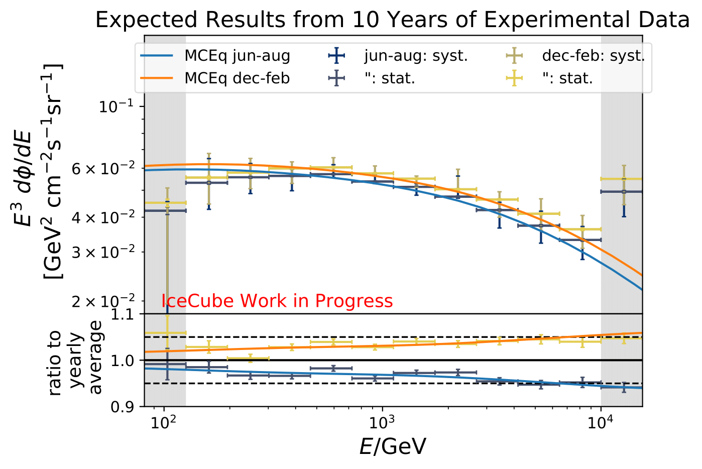
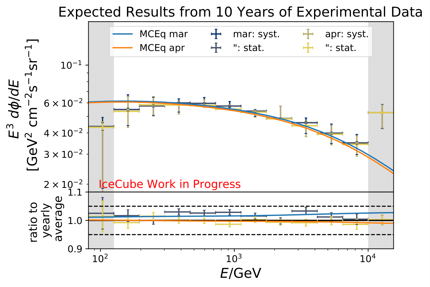
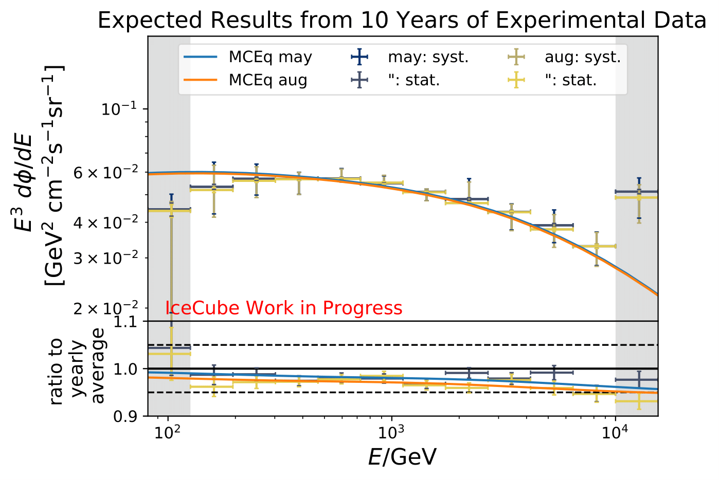
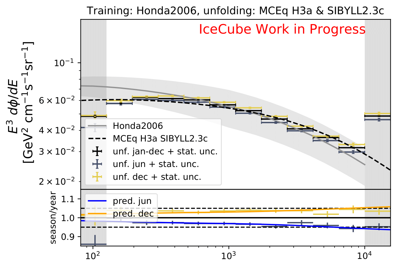
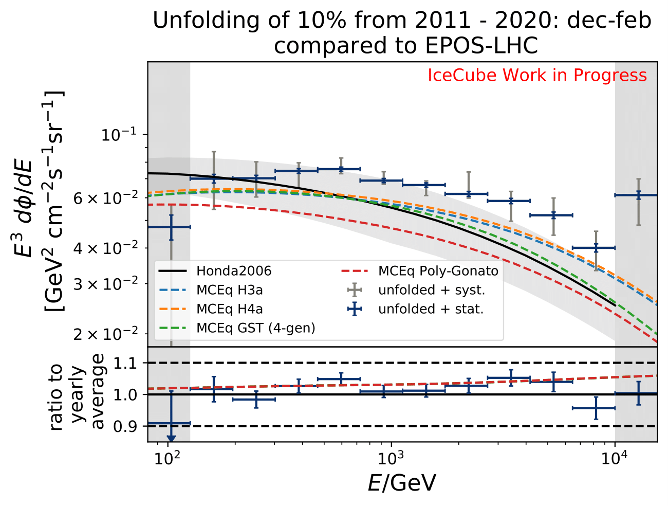
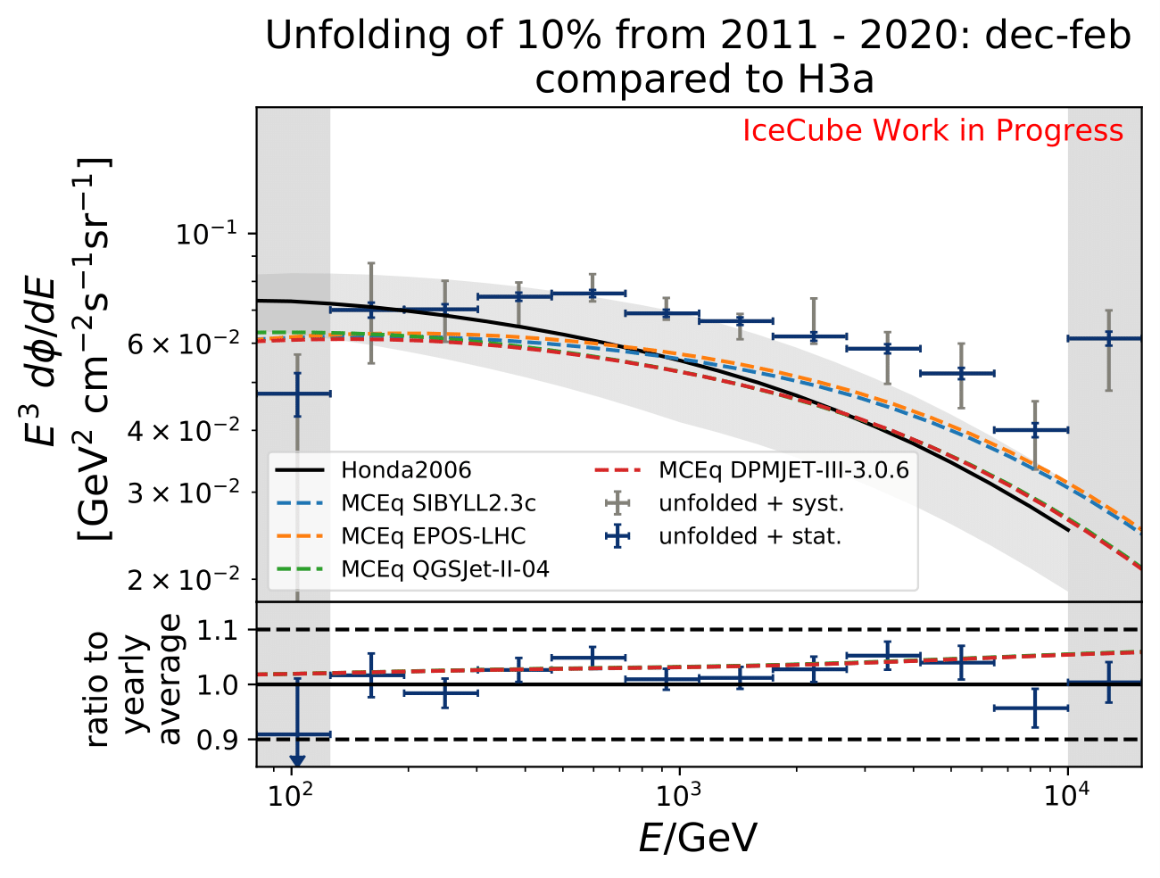
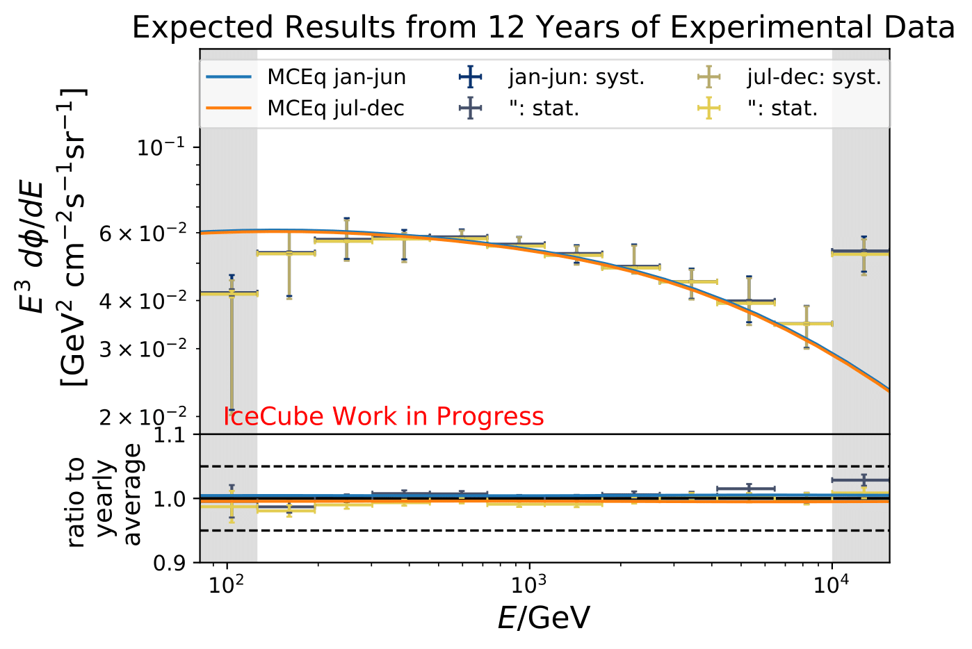
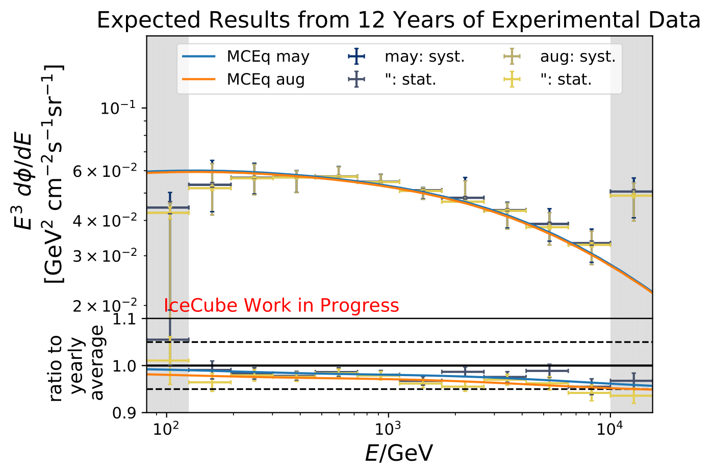
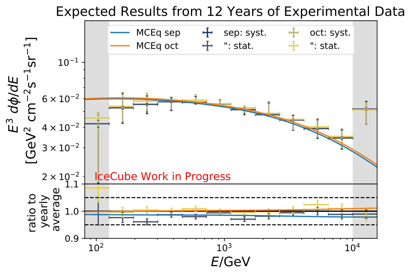
Each of the unfolded spectra is plotted with the corresponding systematic and statistical uncertainties. The systematic uncertainty calculation is a conservative approach and might lead to an overestimation of the uncertainty. The seasonal spectra cannot be distinguished due to the large systematic uncertainties that arise from the detector simulation and event reconstruction. The idea here is that the obtained systematics are independent on the season, as shown in the previous section on systematics. Since the goal of this analysis is to measure seasonal variations, and hence the flux deviation of a specific season towards the annual average flux, the unfolded seasonal flux can be divided by the unfolded annual average flux. This is displayed in the ratio plot on the bottom. The assumption that systematics are seasonally independent (reconstruction and flux model uncertainties), the systematic uncertainties cancel out in the ratio of seasonal to annual average flux. This leaves the flxu ratio only being dependent on the statistical uncertainty of the seasonal and annual average flux, for which both are only impacted by the number of events in the seasonal sample. This uncertainty is expected to decrease with an increasing number of events in the samples. The dashed lines in the ratio plot in the bottom denote +/- 5% deviations from annual average flux. The Honda flux is taken from the paper and is numu + antinumu flux from 90°-120° averaged over this zenith region.

The unfolded seasonal spectra are indistinguishable with respect to systematic uncertainties. The unfolded fluxes are slightly larger compared to the MCEq flux using H3a and SIBYLL2.3c, but are in agreement considering uncertainties in normalization of atmospheric flux. The reason for this could be explained with the data-MC-agreement. Each variable should a data excess over MC of around 20% which denotes roughly the deviation from the unfolded spectrum to MCEq theory flux.

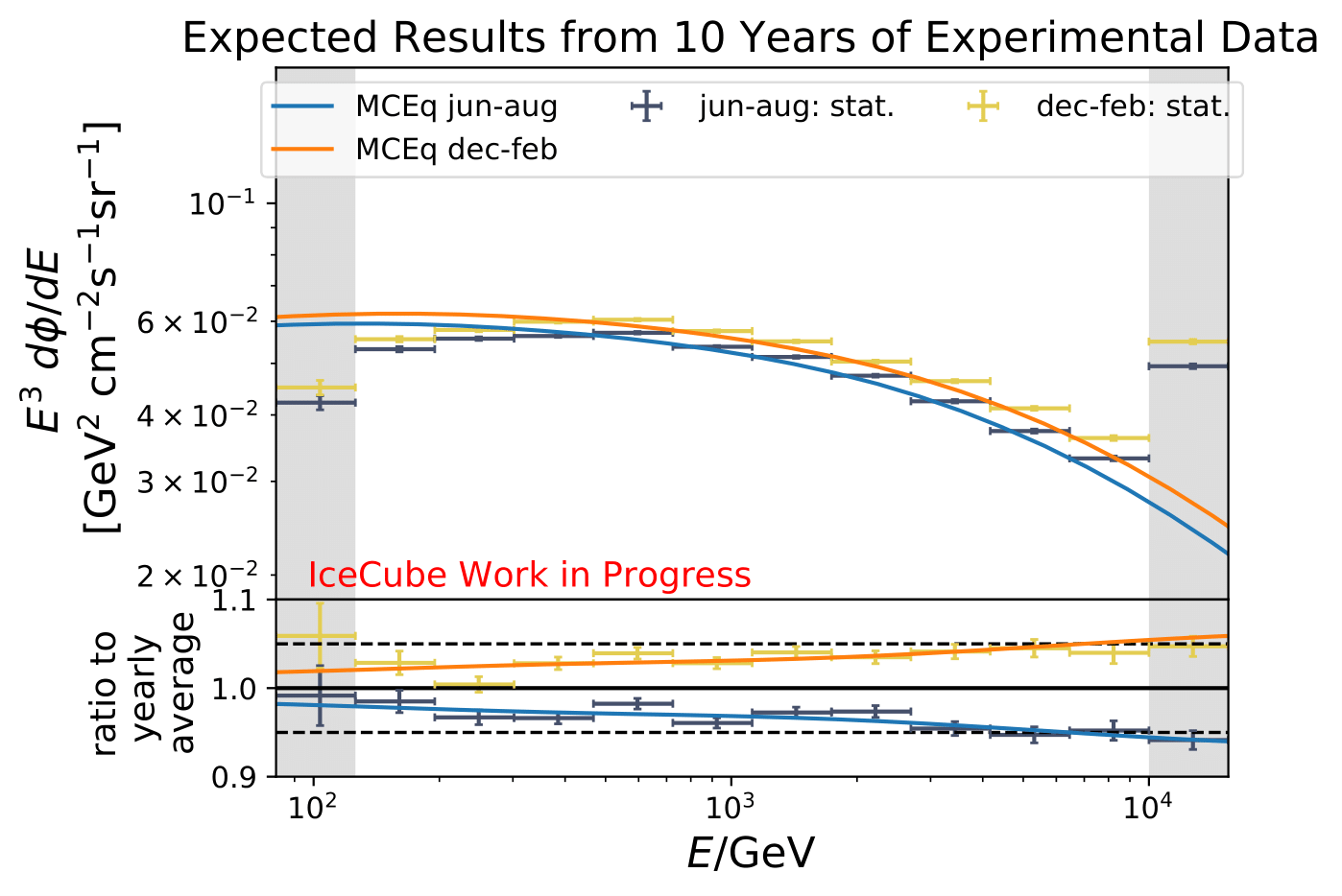
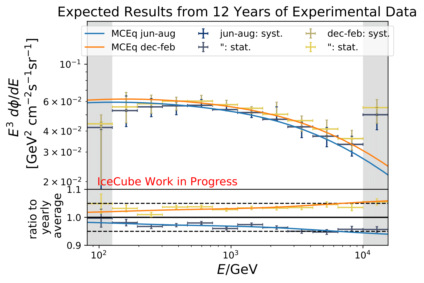
Regarding the unfolded ratio for June to August compared to flux ratio of December to February the flux deviates from the annual mean flux. The variations increase with energy as it is expected from theory. The statistical uncertainty are quite large because only 10% of the available data are used so far. Despite that, a tendency of an increased flux in the season from December to February, as well as a decreased flux for June to August is observable.

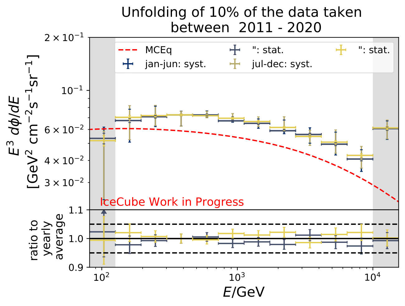
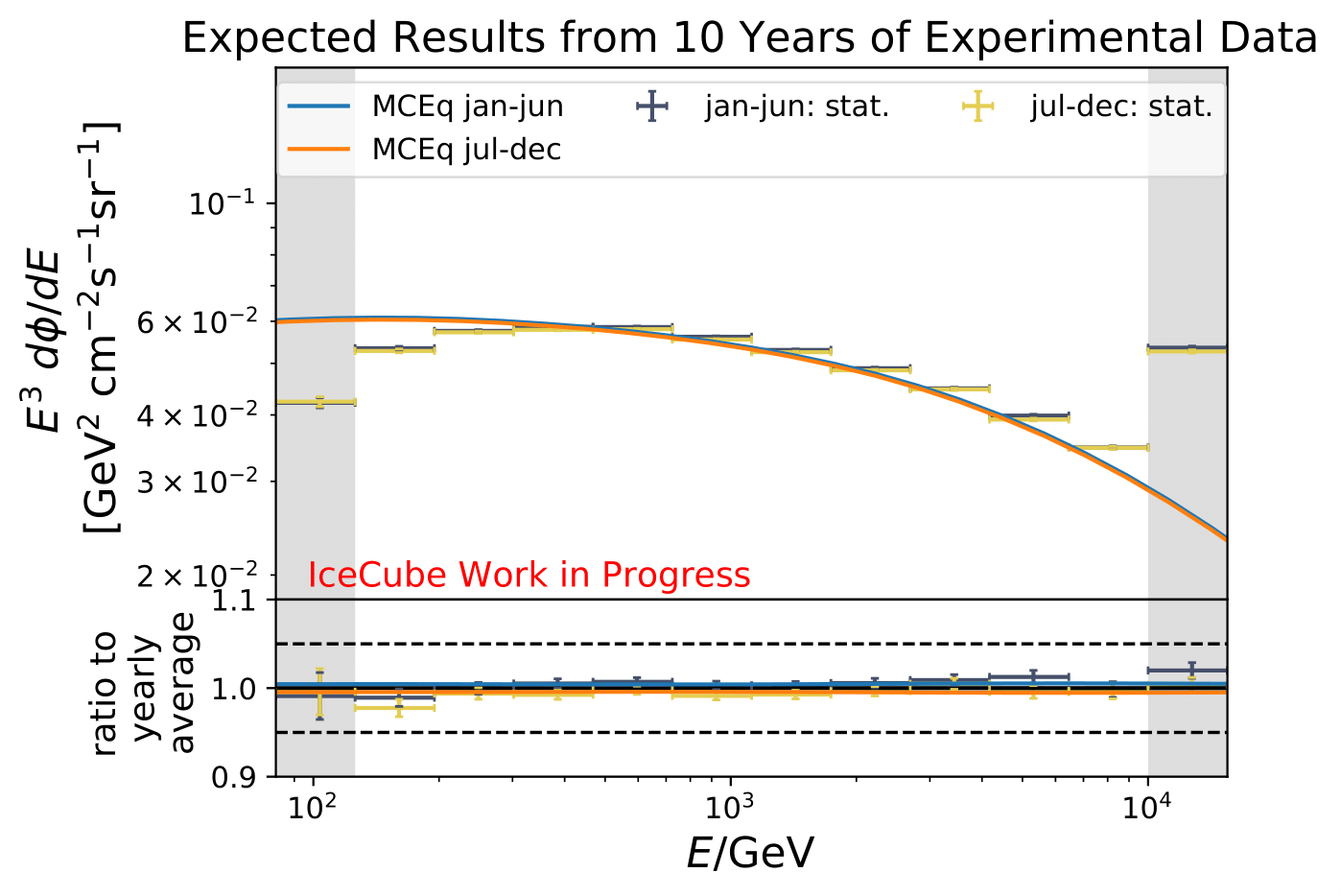
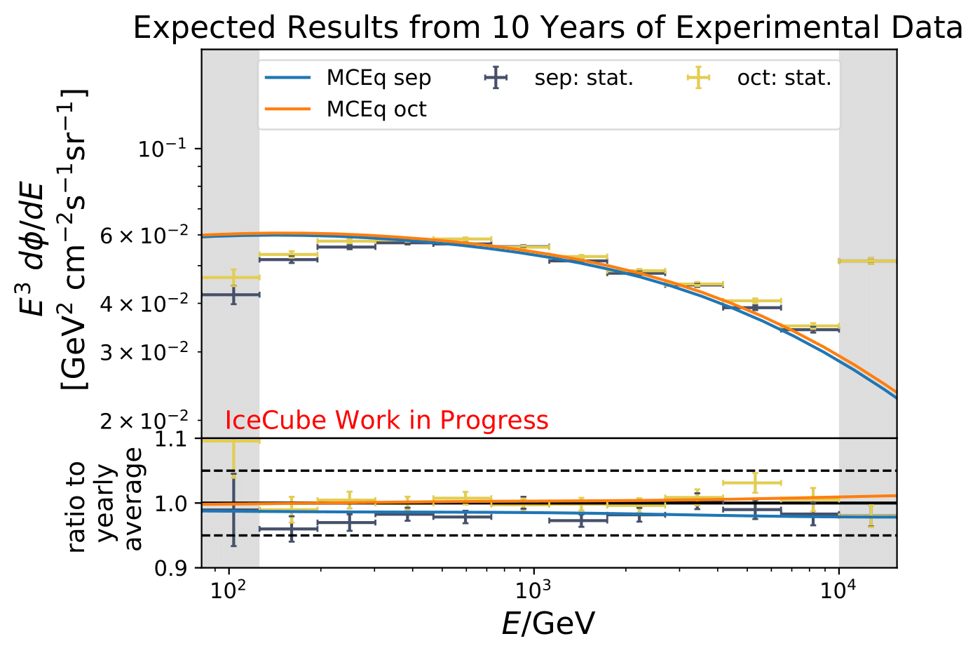
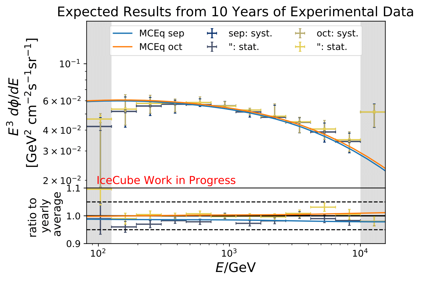
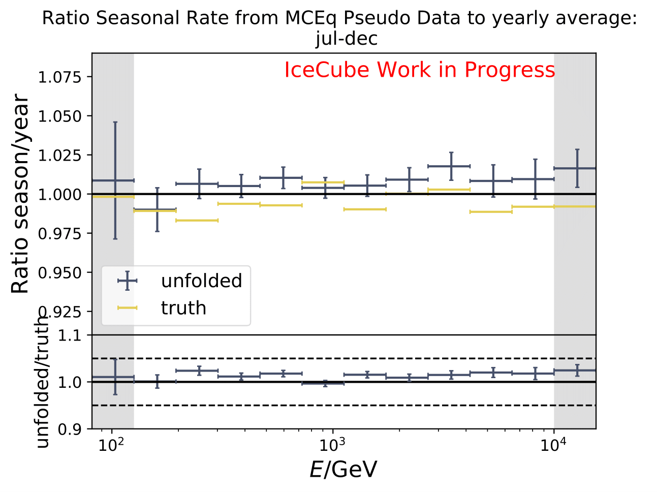
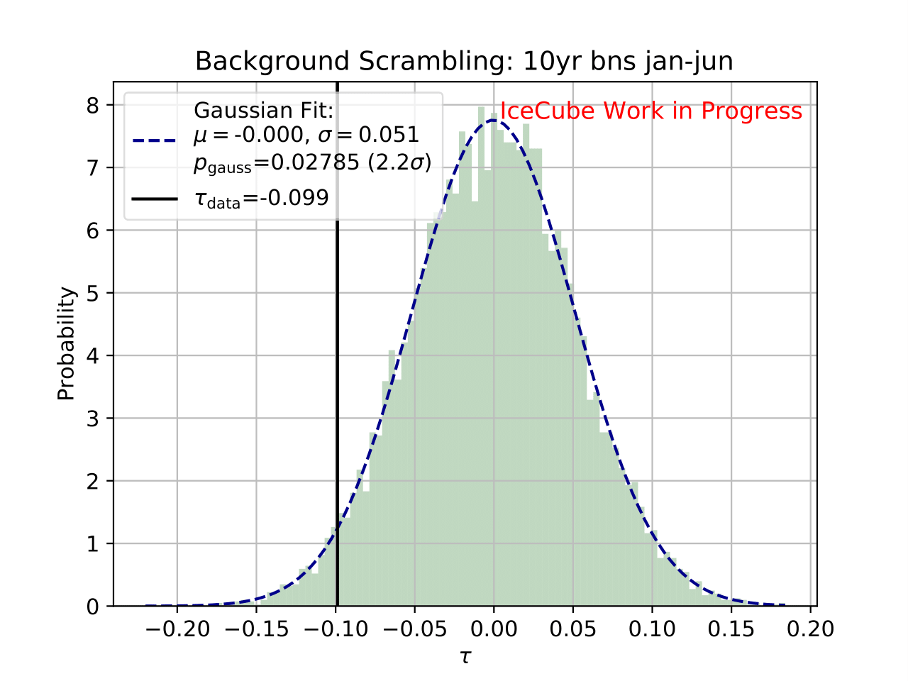
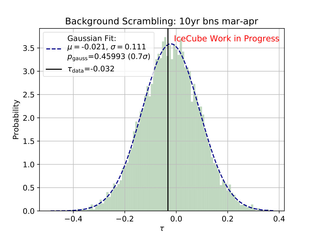
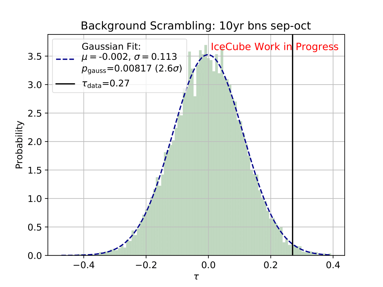
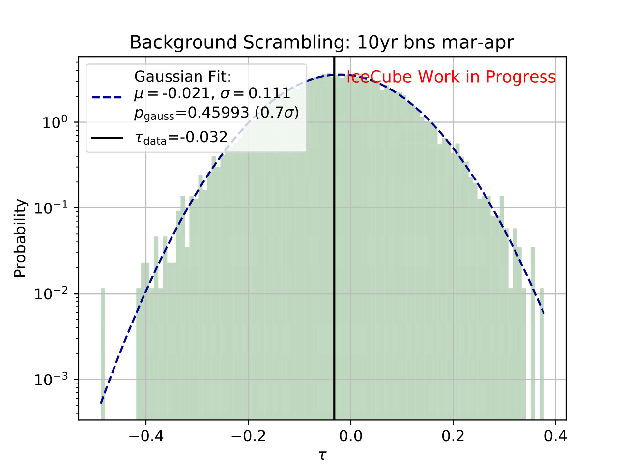
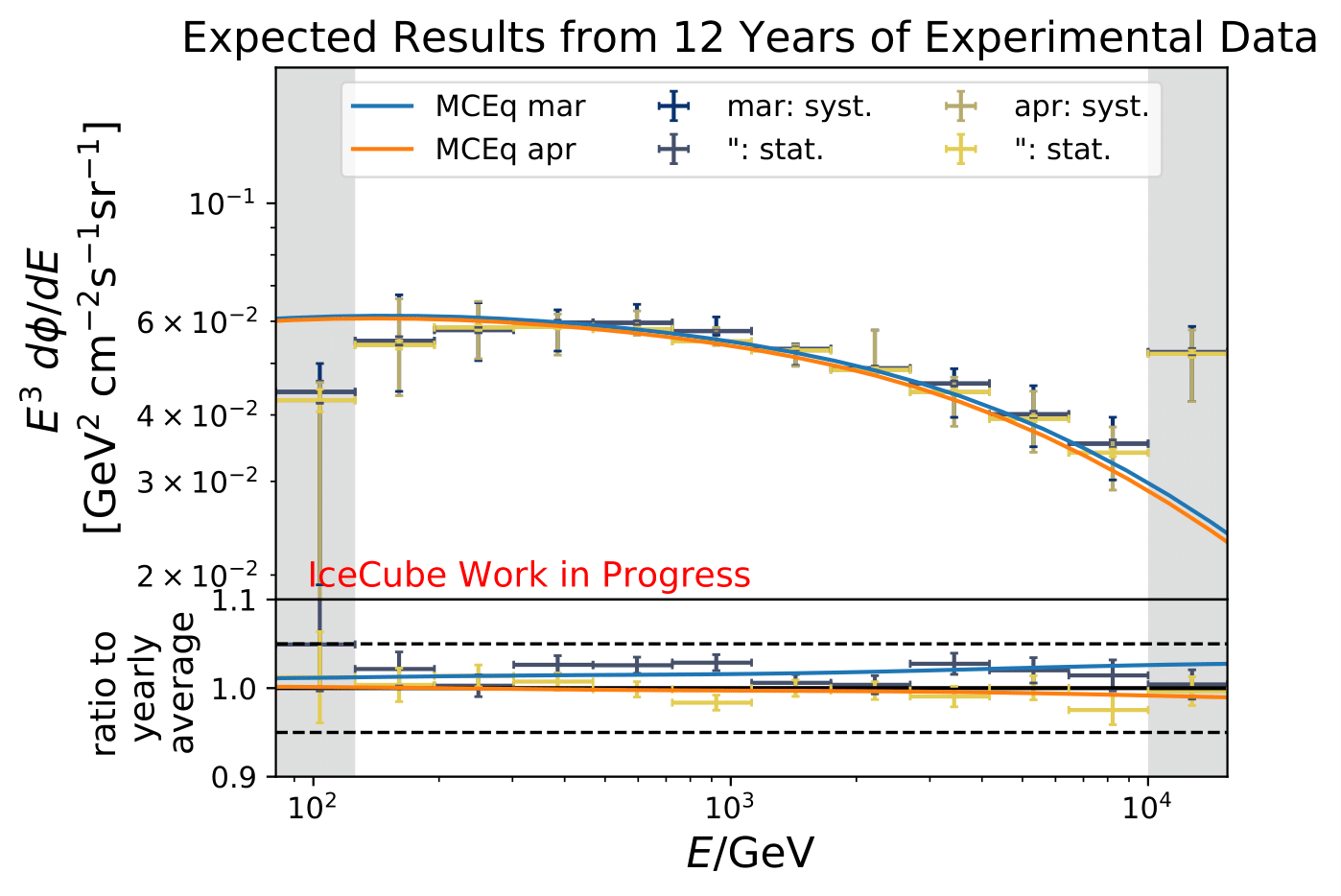
As a crosscheck two additional comparisons are made. Seasons which have similar temperature profiles should not show any seasonal variations and hence be compatible with the annual mean flux. This is illustrated below for the autumn and spring seasons (March-April and September-October). In addition to that, the unfolded flux for the seasons January to June and July to December is compared to the annual mean flux. Both seasons should be compatible with one another.

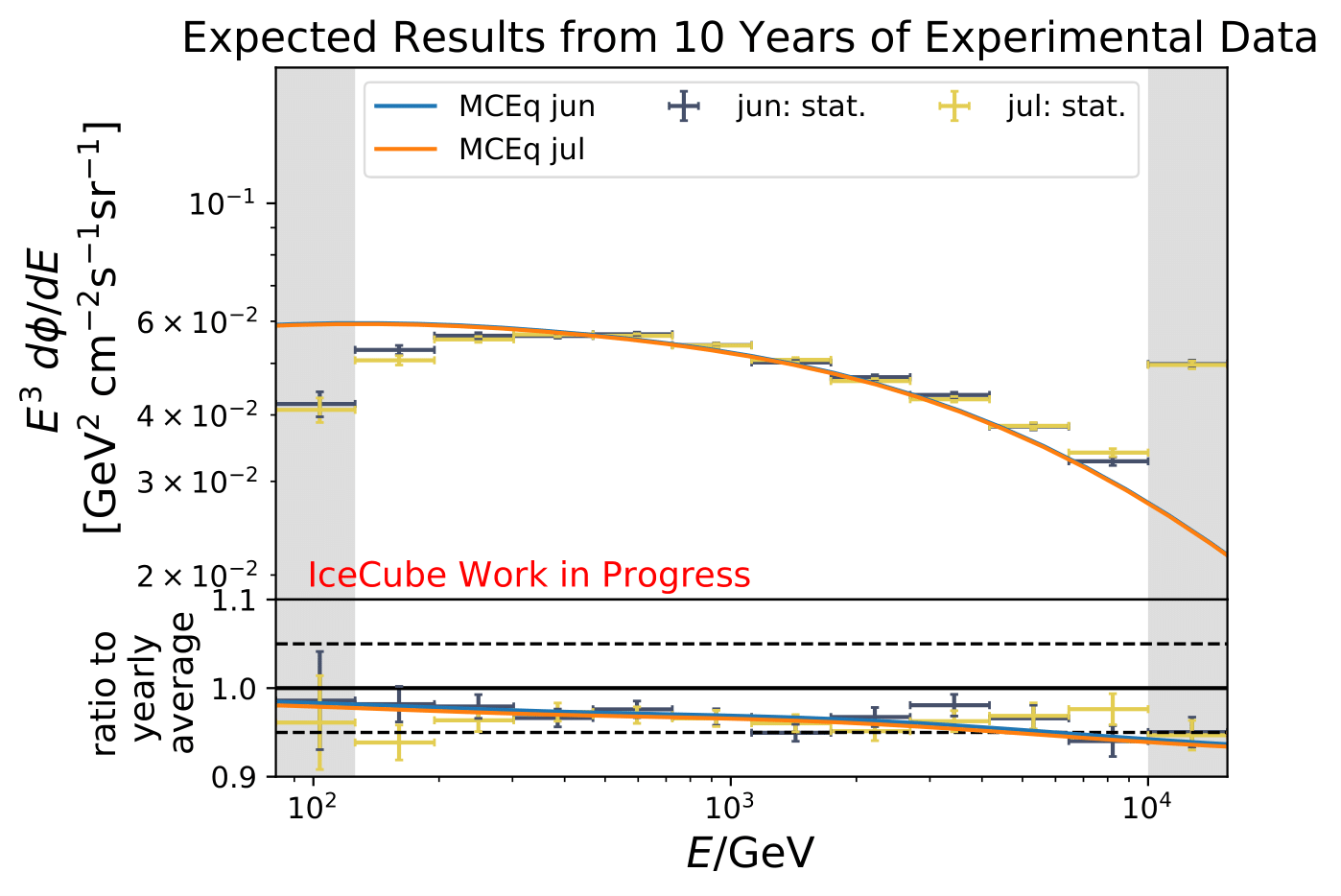
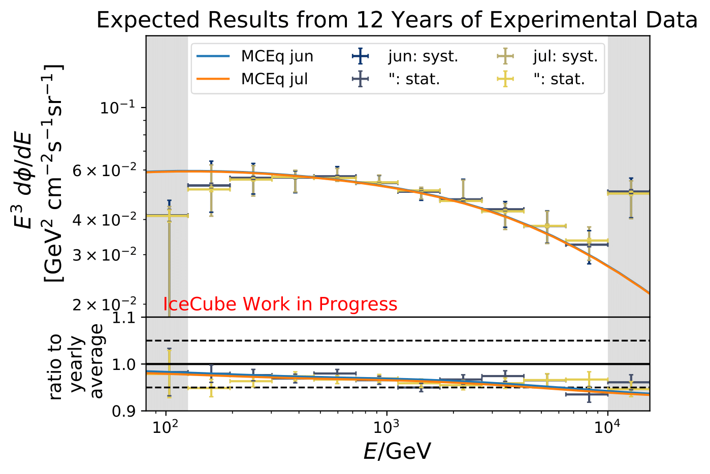
In principle, it would be interesting to investigate seasonal variations for monthly data sets. However, this is not feasible on the limited number of events in the burn sample since the statistical uncertainties would increase tremendously (only very few events are sorted into the highest bins). This could be one possibility to investigate this effect further on the complete data set.

Remark on uncertainty:

The uncertainty of the flux ratio of a season to annual average does not consider correlation between seasonal and yearly data set unfolding in the uncertainty propagation formula. The correlation term will be added after unblinding to ensure the correct calculation. As shown in the Q&A section, the correlation term has no impact on the uncertainties visible in the plot. It was agreed that the plots shown here (burnsample unfolding) do not need to be updated for this reason.

Remark on offset to MCEq:

The unfolded spectra show a constant offset compared to MCEq. The same behavior is observable in the comparison to MCEq with varied primary cosmic ray composition and hadronic interaction models. This offset cannot be incorporated in flux model uncertainties and is already visible in the data-MC agreement. This offset is a common observation in many diffuse analyses. However, this offset is usually governed within nuisance parameter such as the conventional atmospheric flux normalization which is scaled in forward-folding fits towards the data. In unfolding no such treatment is possible. This offset can only originate from the effective area normalization, which is transferring the unfolded event rate into a differential flux. This points to uncertainty in IceCube simulation and can be handled by adding an additional uncertainty on the effective area. The offset is visible more clearly when the flux is scaled by \(E^3\), which is used to make seasonal difference visible. However, the offset is not as evidently observable in the usual scaling by \(E^2\).

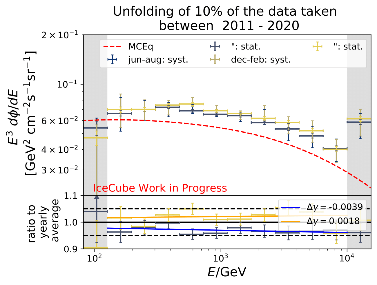
The fits in the ratio plot determine the shift in the spectral index compared to the annual average flux. As can be seen in Q&A section, this was requested as a follow-up within the collaboration review. A simple power law is fitted to the unfolded ratio including the uncertainties in the fit. The fits will be obtained on the monthly unfolded samples after unblinding is permitted.

Comparison to diffuse 3yr unfolding (no uncertainties are shown for the 3 yr diffuse unfolding - zenith: 86°-180°):

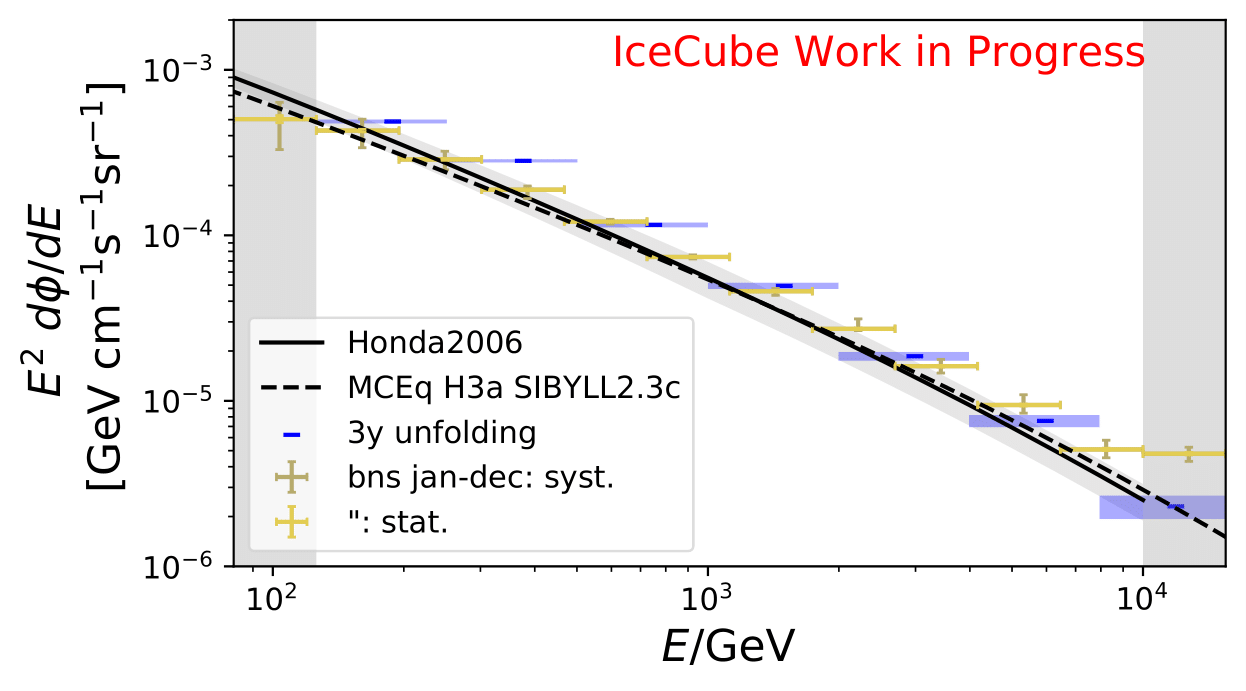
Honda flux and MCEq are shown for the zenith range of 90°-120° and yearly average flux. The 3yr unfolded flux is in agreement with the burn sample unfolding for jan-dec. The zenith range for the 3yr unfolding is 86°-180°.

Rate Comparison

10yr sample:

Seasonal Burn Sample before and after unfolding

Season	Rate before [1/d]	Rate after [1/d]	Events
jun-aug	120.8	120.8 +/- 0.8	10682
dec-feb	127.0	127.0 +/- 0.9	10574
jan-jun	123.6	123.5 +/- 0.6	21532
jul-dec	125.5	125.5 +/- 0.6	22172
mar-apr	124.4	124.4 +/- 1.0	7563
sep-oct	127.7	127.7 +/- 1.1	7683
jan-dec	124.5	124.5 +/- 0.4	43704

Estimation of Full Sample Results

The ability to measure seasonal variations energy-dependently with an unfolding technique is tested using the weighted MC sample. Pseudo-data are generated by weighting the MC simulation to the seasonal predictions from MCEq (H3a, SIBYLL2.3c). Number of events corresponds to number of events in burn sample multiplied by factor 10 to resemble the expected number of events in full sample. This number has to be set accordingly to have a trustworthy estimate of the statistical uncertainty. The livetime is obtained from the MC and is given by the sum of the seasonal weights.

The seasonal weights are calculated based on the average of the monthly fluxes. The annual average is given by the conventional flux, the average of the monthly fluxes.

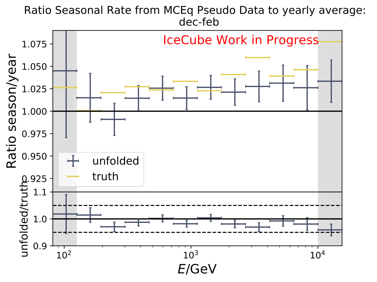
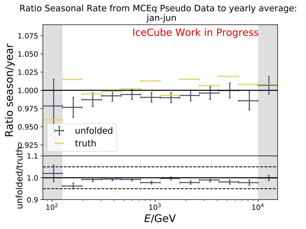
Reminder: the following plots contain statistical uncertainties only. This uncertainty originates from bootstrapping the data set, but does not contain systematic uncertainties of the algorithm.

The following plots contain statistical and systematic uncertainties:

The ratios obtained from unfolding are in agreement with the MCEq prediction. The effective area matches the unfolded pseudo-data in normalization and shape.

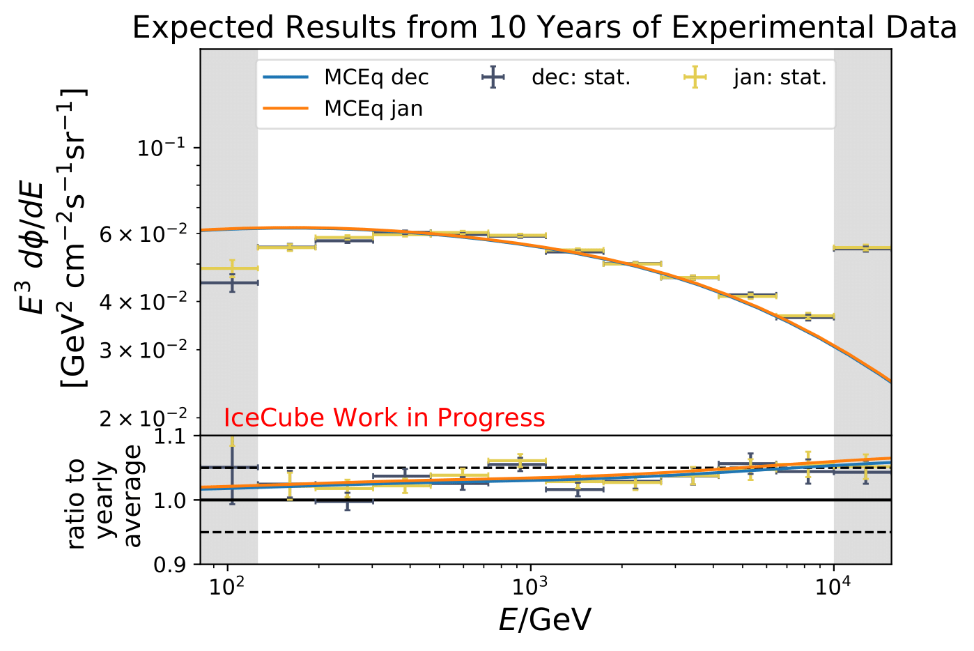
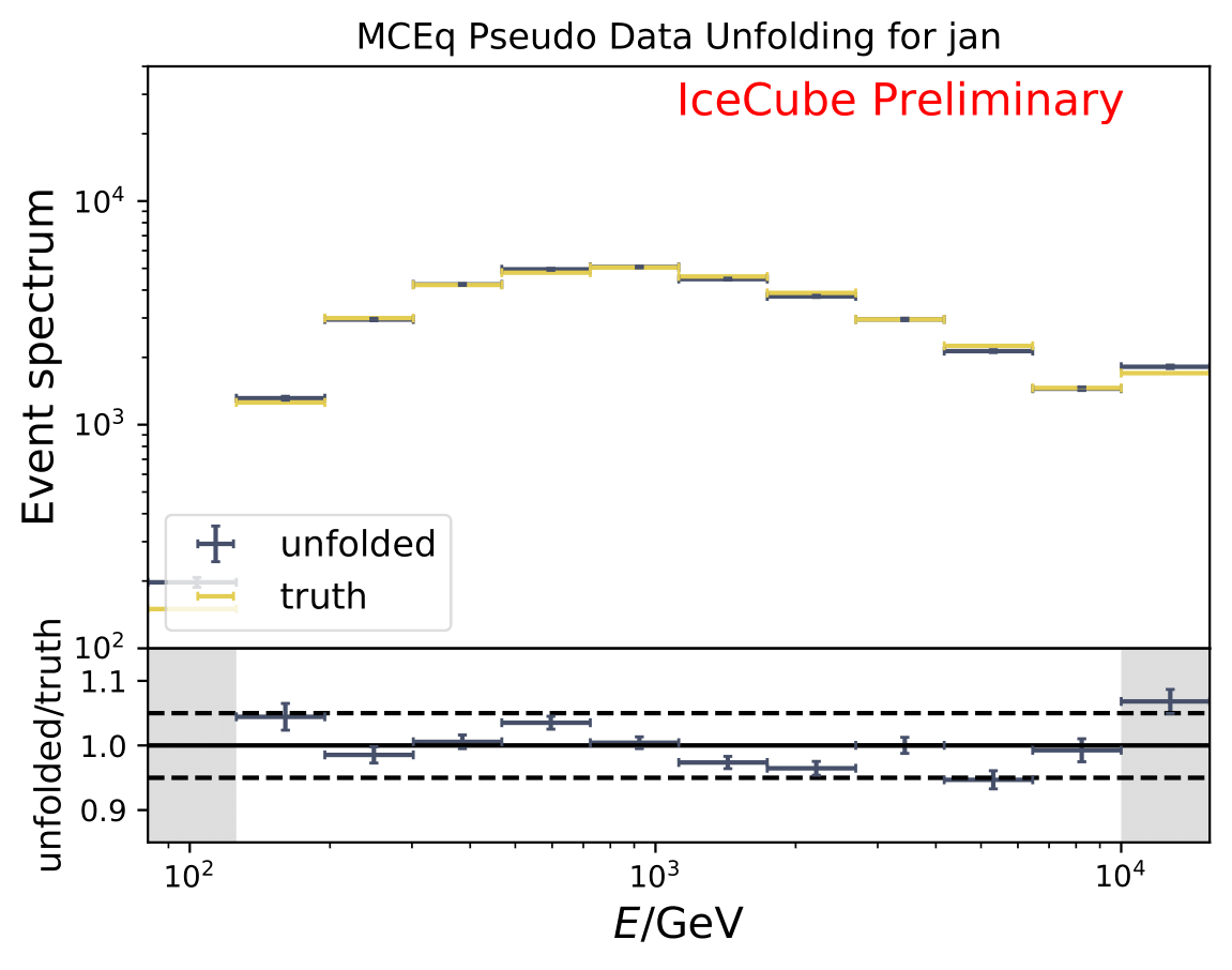
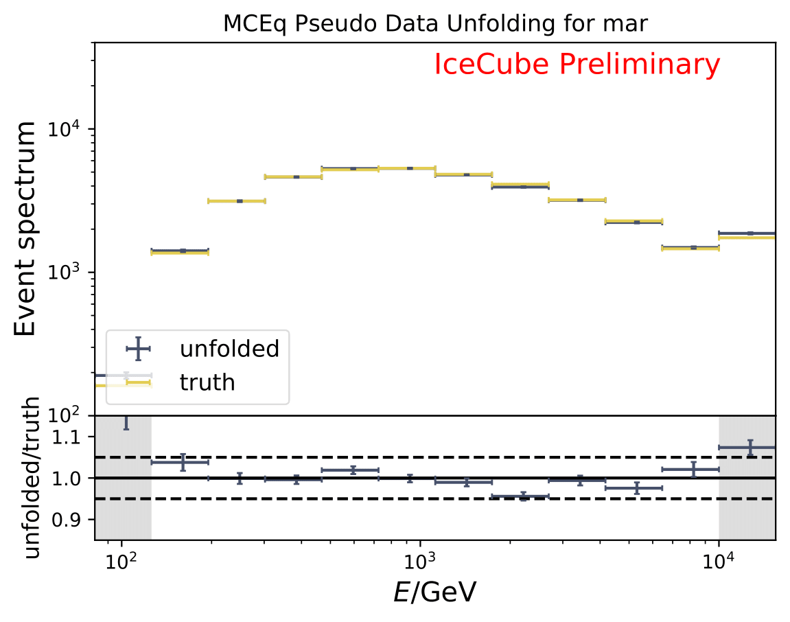
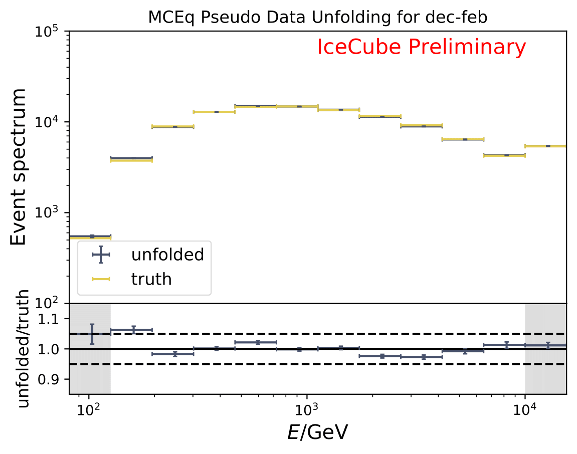
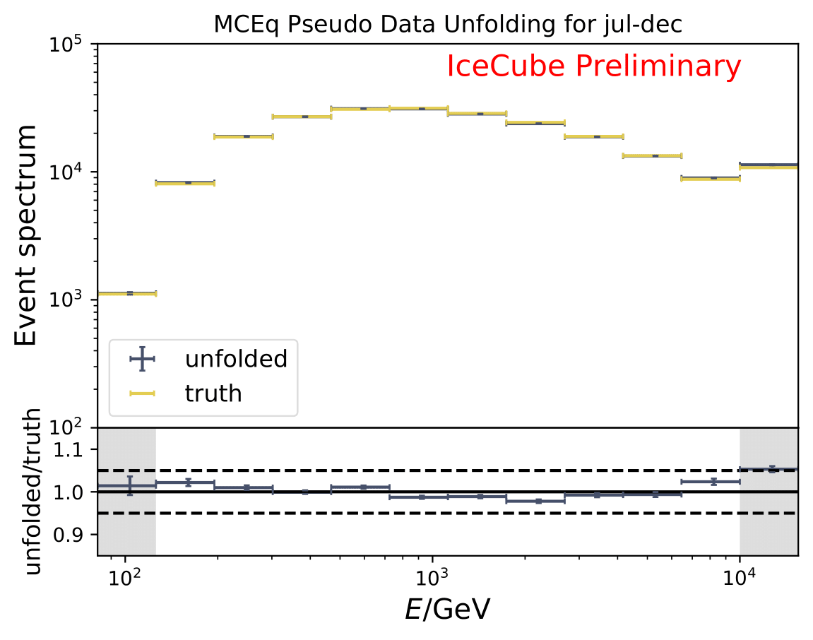
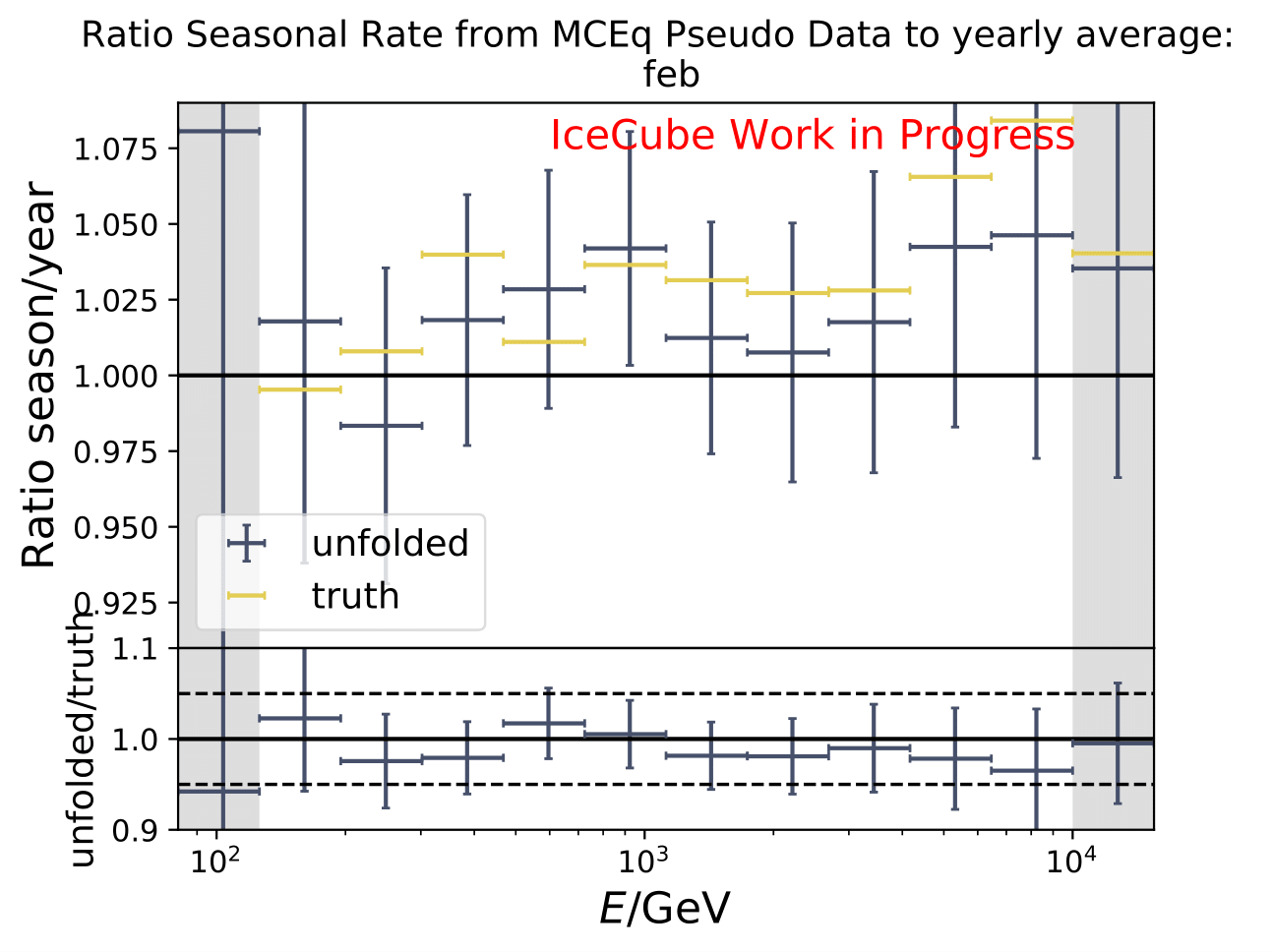
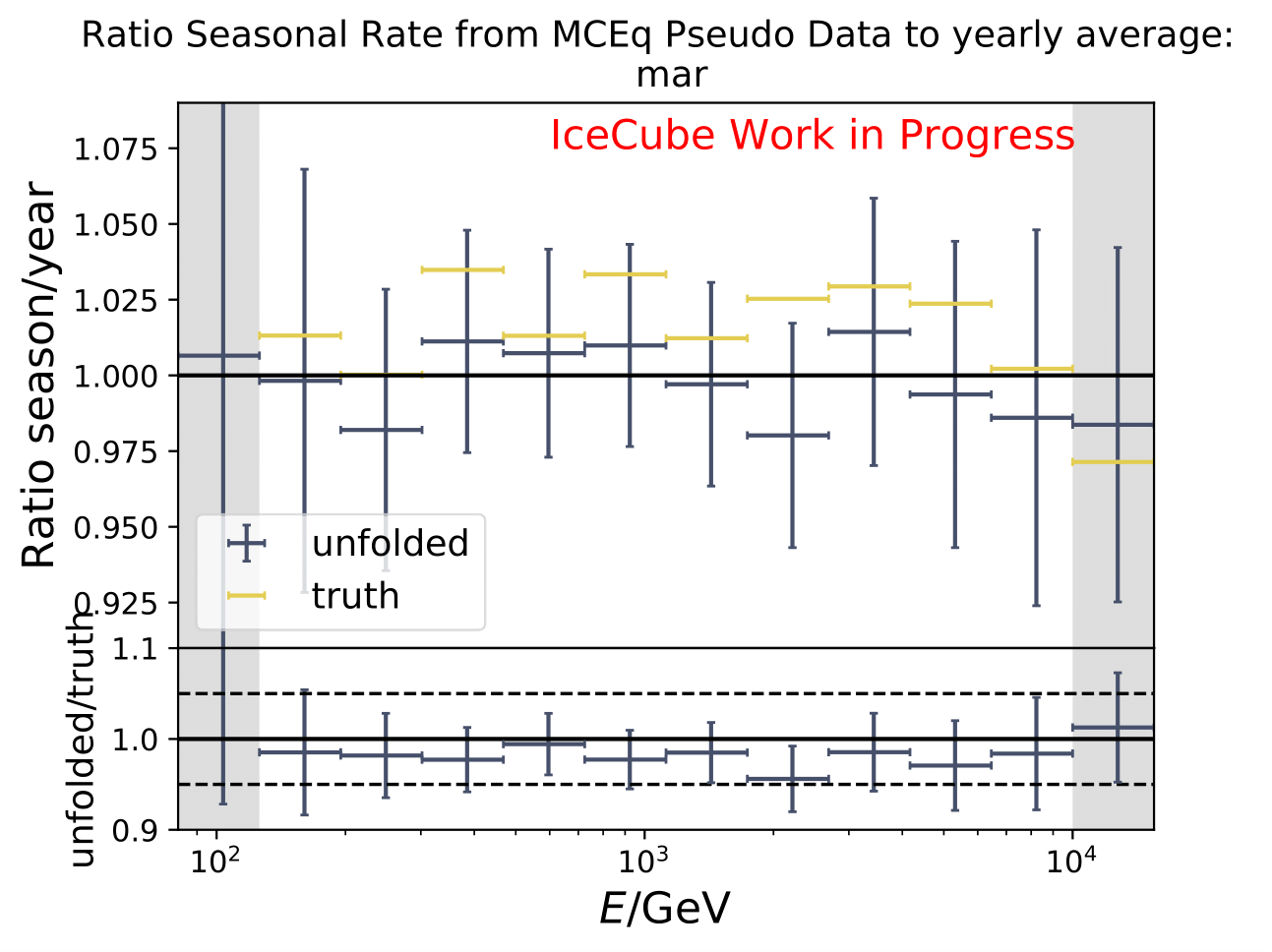
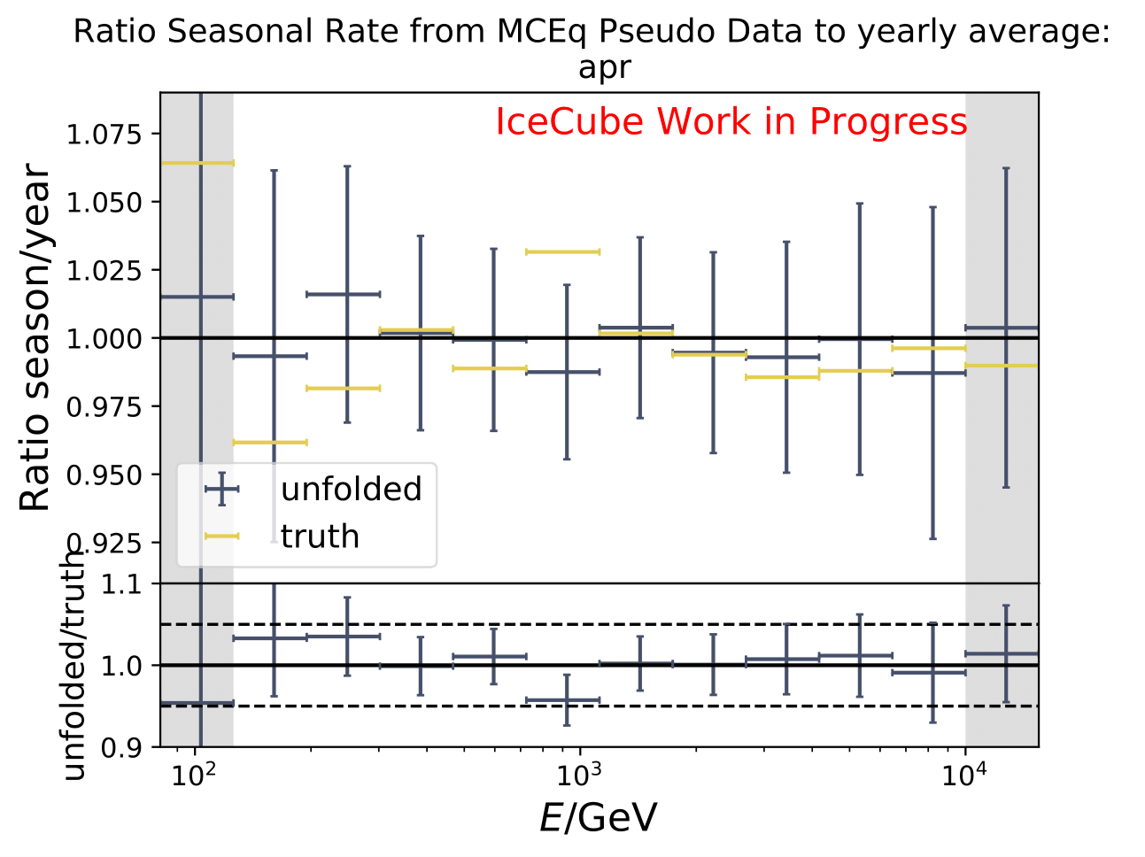
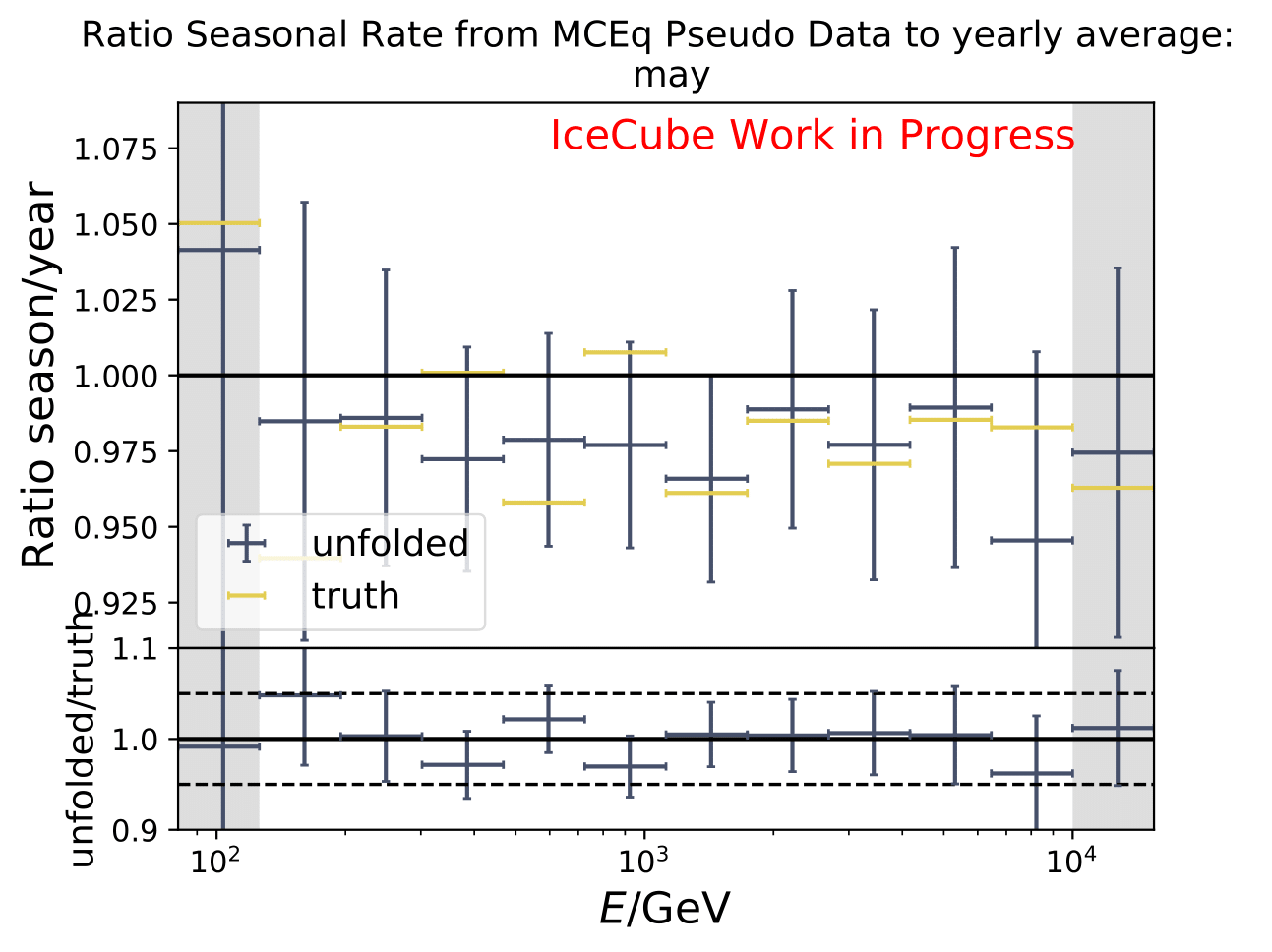
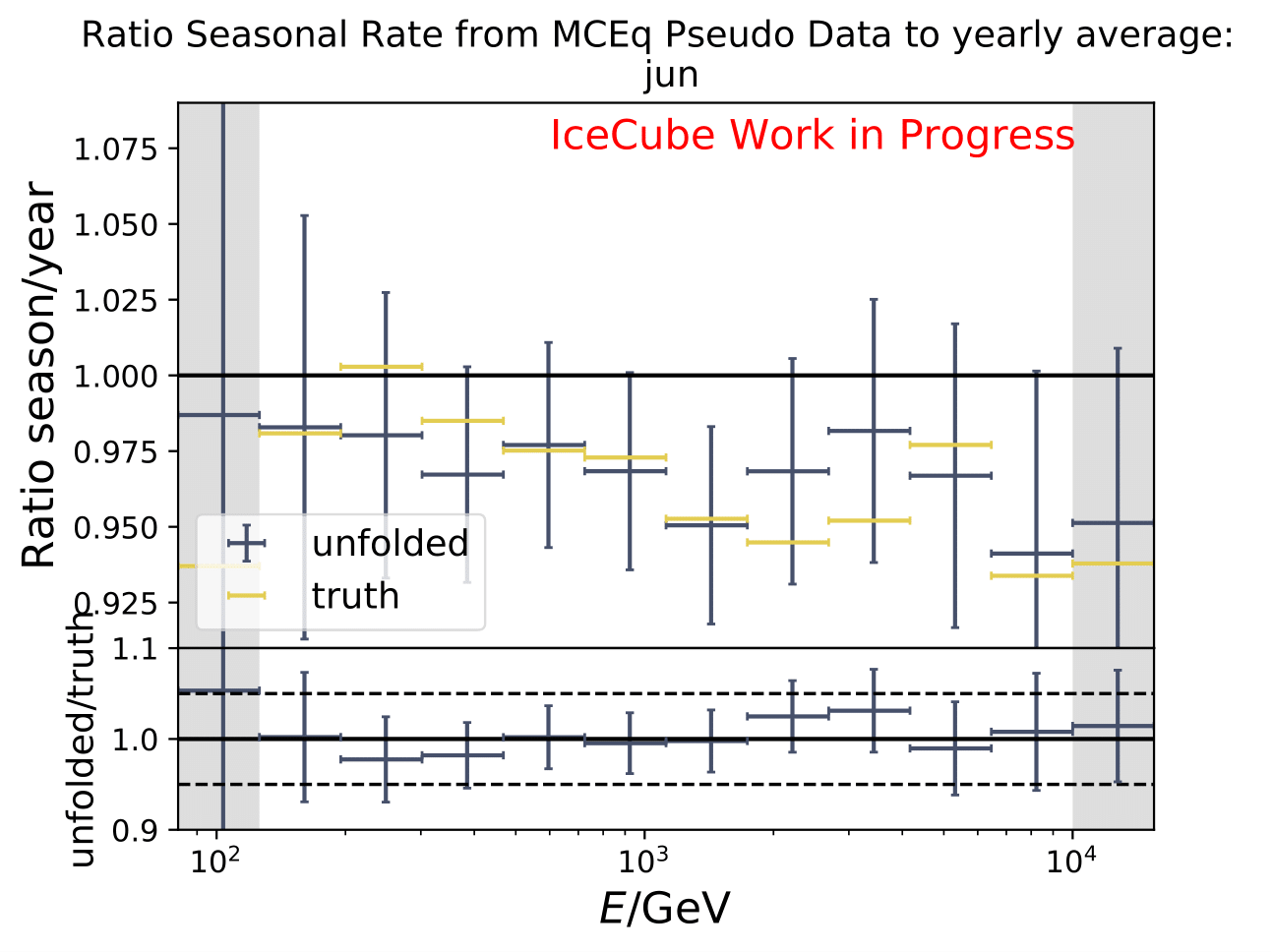
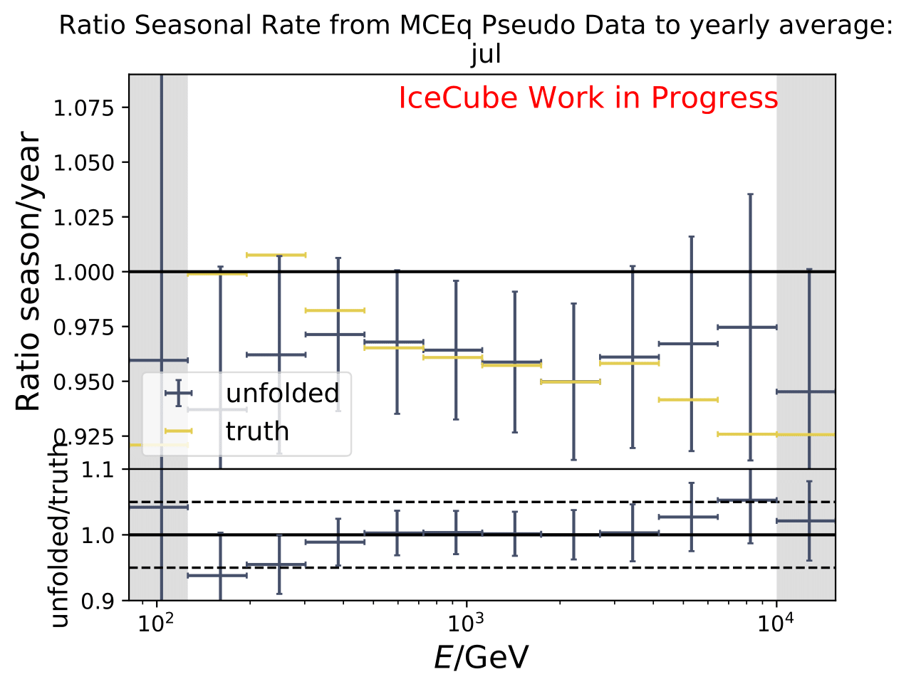
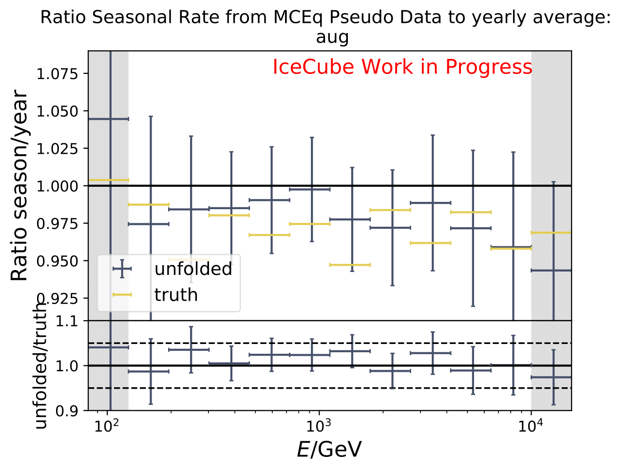
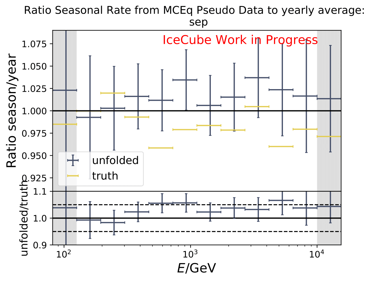
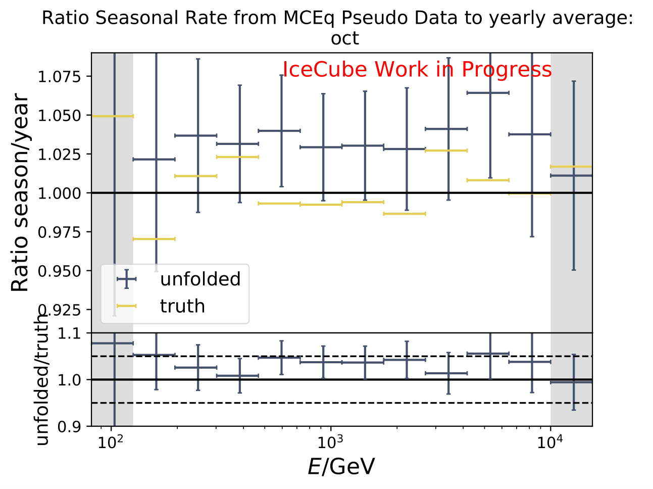
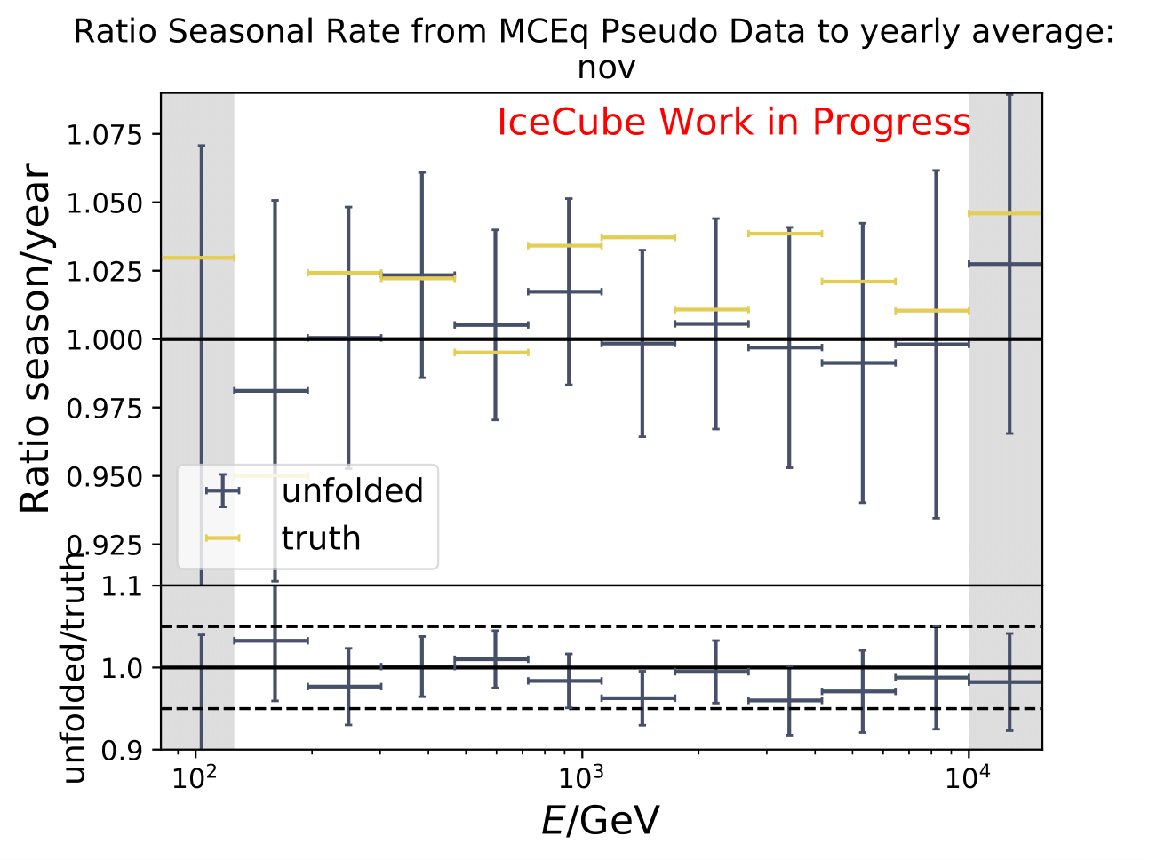
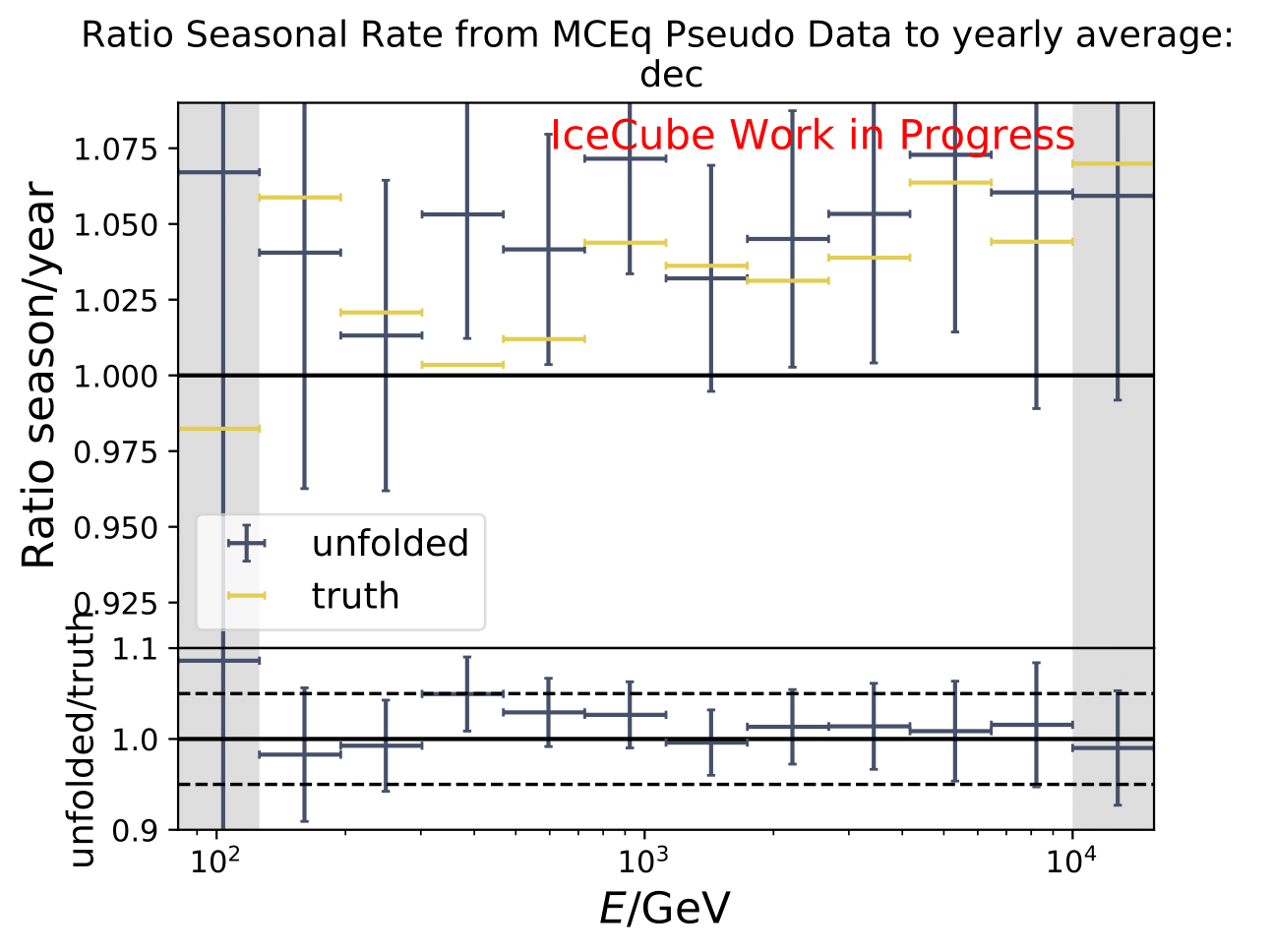
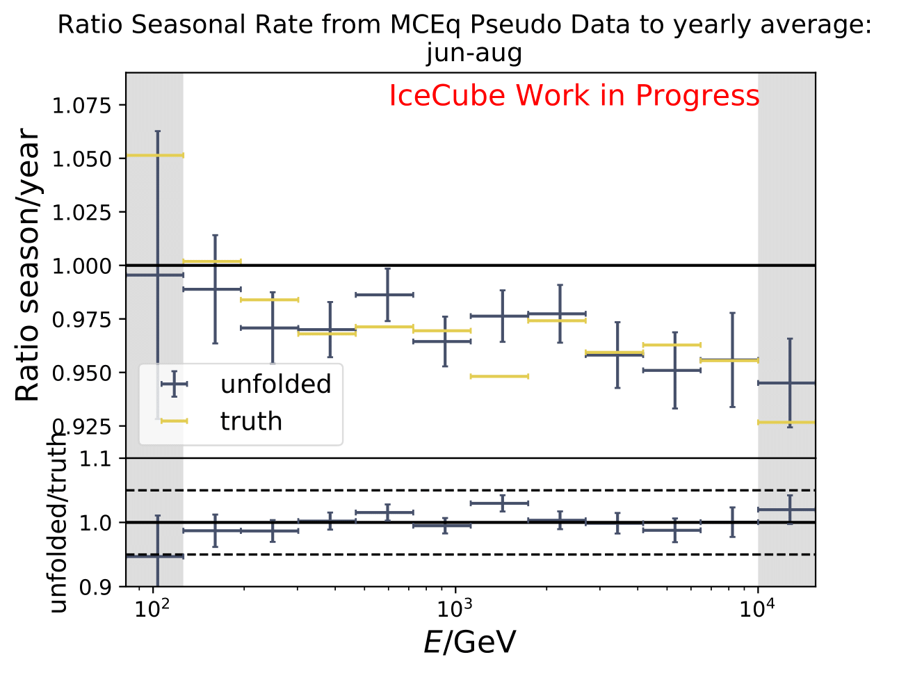
The next test determines how well the truth can be determined by the unfolding. The plots depict the true and the unfolded event spectra for each month. The number of events from the burn sample is scaled up by a factor of 10 to display the estimation of the full data set. The uncertainties correspond to statistical uncertainties from unfolding. These plots merely serve for testing purposes. The quantity of interest is how well the ratio of seasonal flux to annual average flux can be determined. These tests are depicted further below.

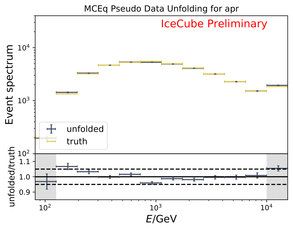
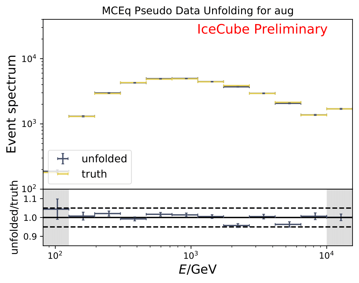
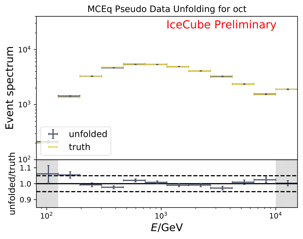
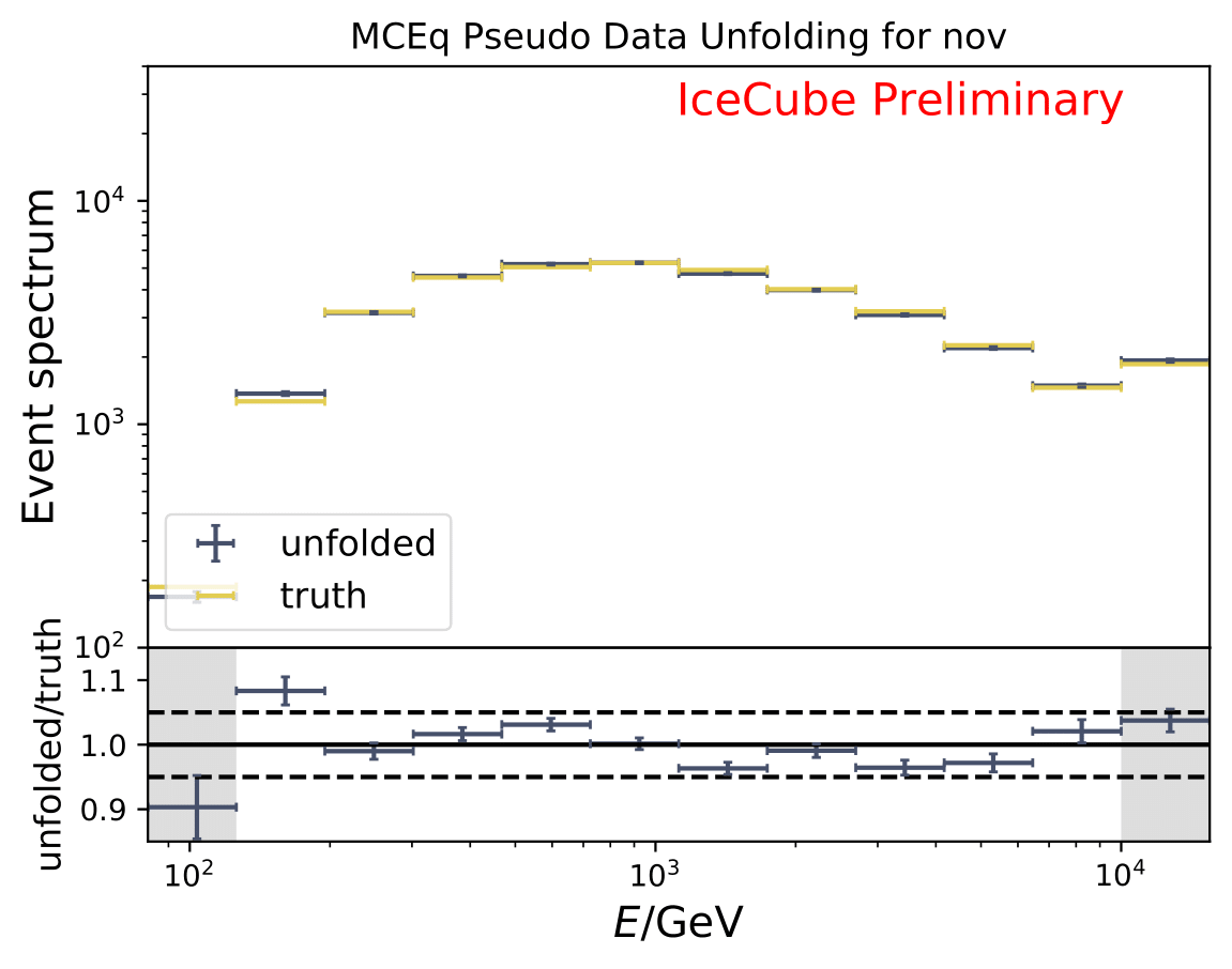
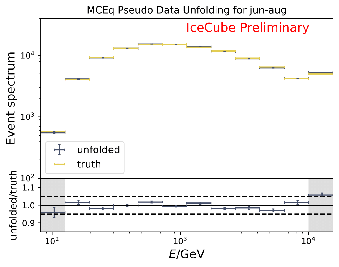
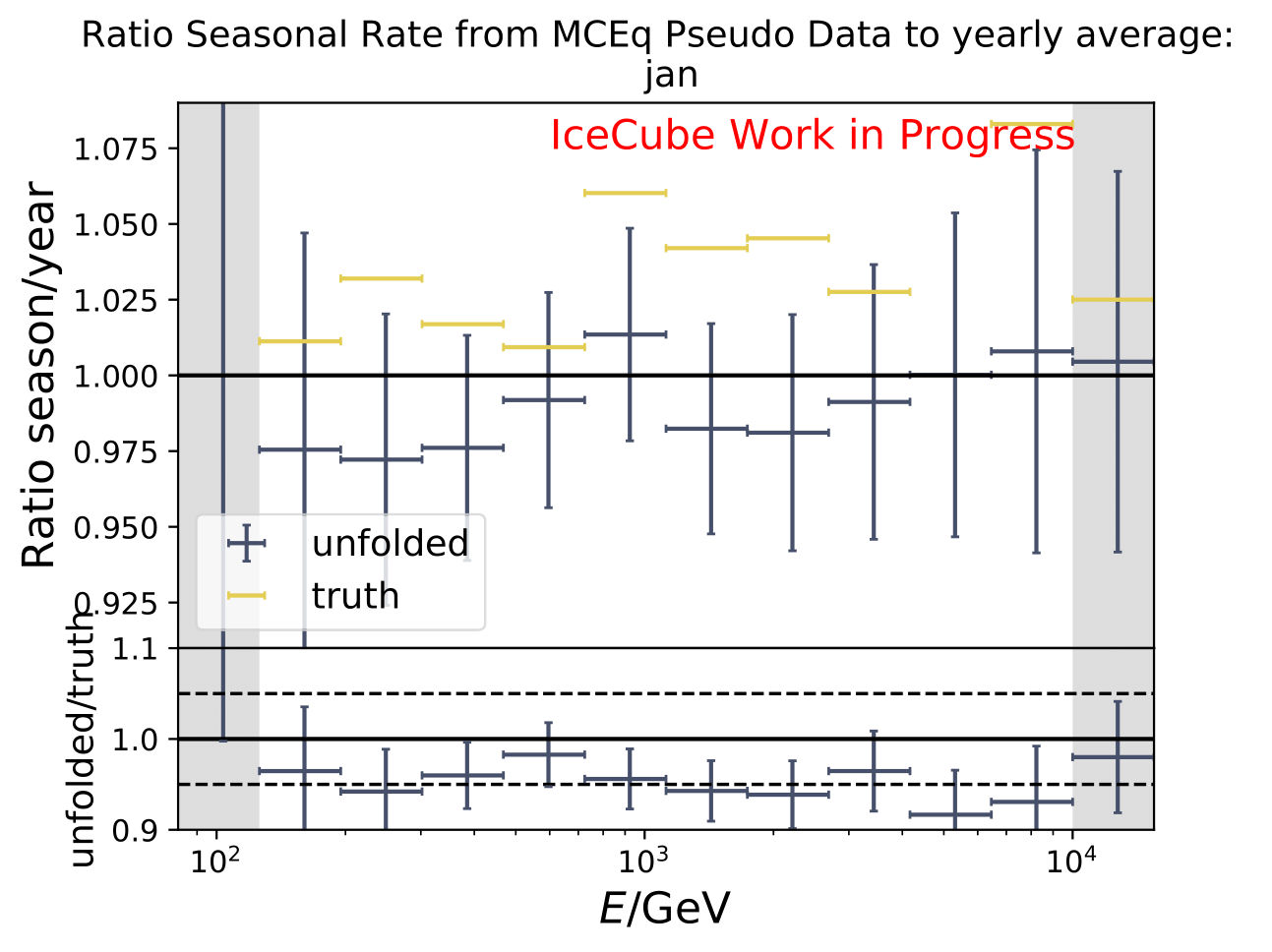
The same test is shown for the ratio of seasonal to annual average flux (quantity of interest). The truth can be well retrieved from the unfolding.

Tests with Honda Flux

It is noticeable that the first bin was underestimated in the MC unfolding round trip test. Unfolding the event spectrum and comparing to the MC truth shows slight deviation in some months especially in the first bins which do not contain much statistics in the training/test sample. However, the ratio of seasonal unfolded to unfolded annual average flux are not impacted. A proposed test to investigate the unfolding behavior is training on MCEq and unfolding Honda2006 weighted MC. Number of events is compatible to the full data set estimation from jan-dec. Red denotes MC truth of Honda2006 model, orange MCEq truth. Unfolding is denoted in blue. The ratio shows unfolding over MC truth for both MCs, one weighted to MCEq and one to Honda2006. Both are shown to determine if the unfolded spectrum is in agreement with the input or the MC truth of the unfolded sample.

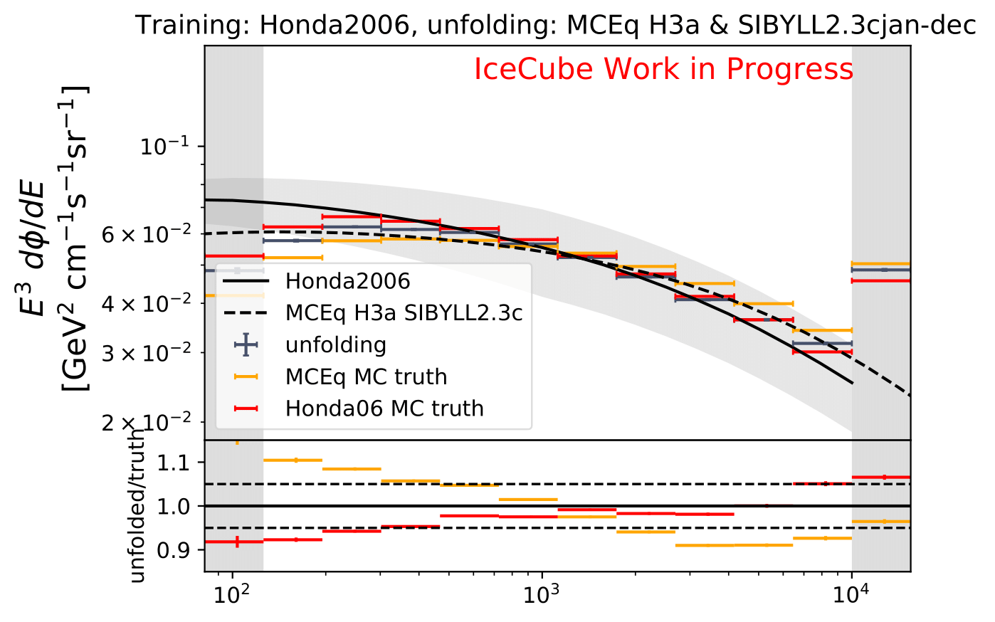
It must be noted that this plot only contains statistical uncertainties which do not repsect systematic uncertainties of the algorithm. These are given in systematic uncertainties and must be added for proper comparison. A systematic shift is visible in the ratio of unfolded to true spectrum. The intermediate energy range around 1 TeV is estimated well, whereas larger deviations around 10% are seen in upper/lower bins. These bins contain few events in both, training and test sample. This is why the unfolded result is closer to the Honda2006 flux on which was trained than the correct flux of MCEq (orange). Same behavior is visible in bin 10. This behavior is already respected in the calculation of systematic uncertainties. The asymmetric error bars (which are not shown in this plot) show a large upper error at low energy bins and a large lower error at high energies. This represents the behavior that is visible in this test. Both spectra can only be compared using systematic uncertainties respect the uncertainty of the DSEA algorithm.

As an opposite test, DSEA is trained on Honda2006 weighted MC (as it was done for Pass1MC) and the MCEq weighted pseudo-samples for the full data set seasonal estimation are unfolded.

The unfolded seasonal spectra (MCEq weighted MC) is shown with statistical uncertainty only without systematic uncertainties of the unfolding. The yearly average in black matches the MCEq predicted yearly average flux in black dashed lines in every bin within statistical uncertainties. Differences between seasons are visible in the spectrum as expected from theory. The change of the training input does not impact the ratio of seasonal unfolded flux to yearly average flux. The ratios are compatible with the prediction from MCEq within statistical uncertainties over the full energy range. The determined result (ratio) is the same as above in the MC unfolding shown in the previous section.

This test is a strong indicator that the unfolding algorithm and the desired target quantity (flux ratios) are robust against changing the input spectrum of DSEA. Comparing the behavior of DSEA when trained on MC weighted to Honda2006 versus MCEq flux can be drawn regarding the Pass1 analysis where Honda2006 flux weights were used to sample the training input. When comparing systematic uncertainties, an increase is visible when DSEA is trained on MCEq weighted MC compared to the old analysis with Honda2006 flux weights. Note the different scaling in the uncertainty plots. DSEA weighted to MCEq shows a larger bias at lower and higher energies than DSEA trained with Honda2006. To determine the reason for this behavior, the training scheme of the algorithm has to be understood. In principle DSEA does not have any information on the input spectrum. Only information given is number of events per bin in the training sample following the given distribution. Bins are treated as independent categories, no spectral information is respected in the algorithm. The random forest predicts a number of events per bin independently. When training with Honda2006 is simply means that the algorithm ‘sees’ more events at lower energies compared to MCEq+astro training. Hence, the algorithm can predict the lower energy bins more reasonably. It should be considered to keep Honda2006 flux as training input because systematic uncertainties would be smaller and the algorithm performs more stable. Another indicator underlining this is the unfolding of Pass2 data but training with Pass1 MC in the old analysis which worked as well.

Significance Calculation

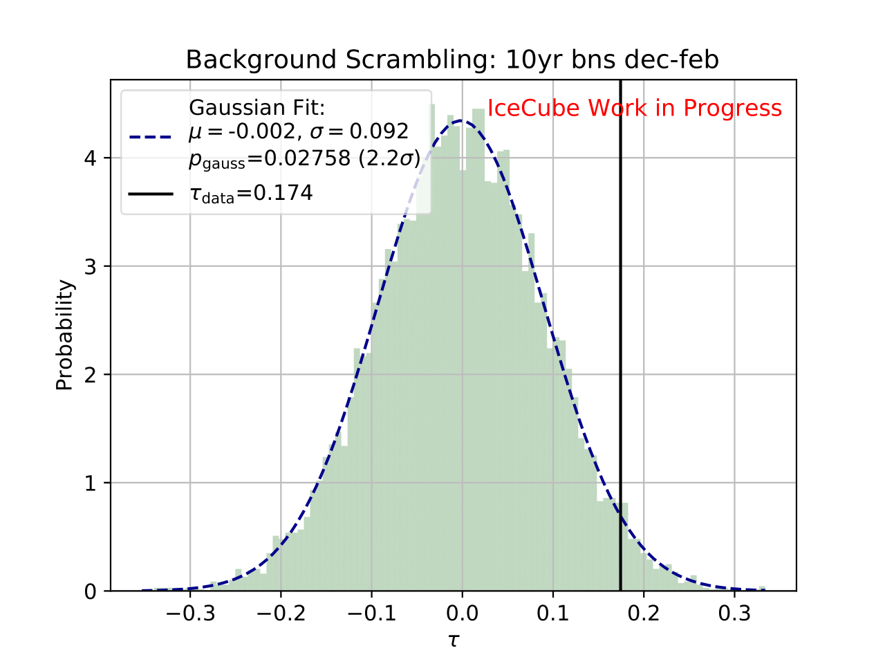
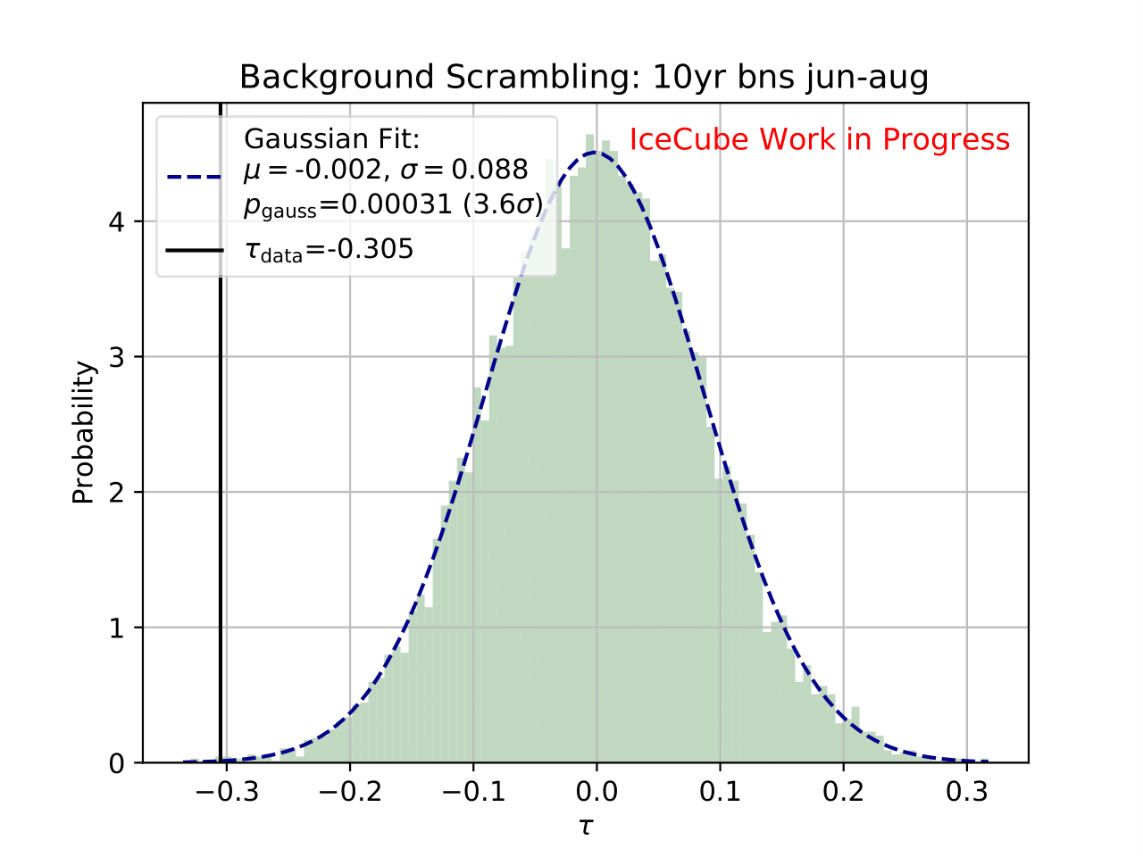
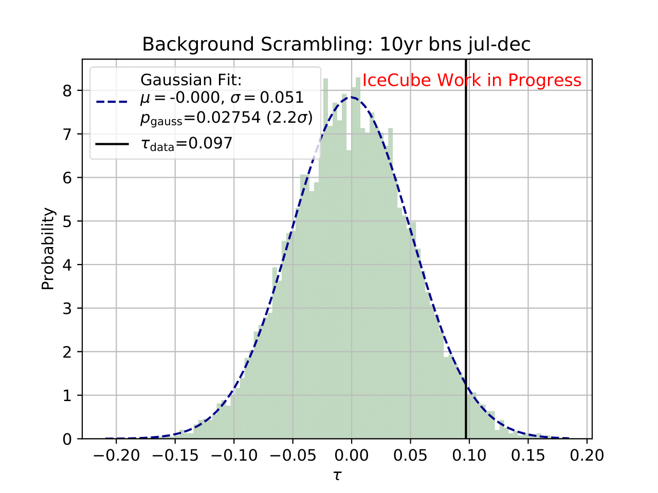
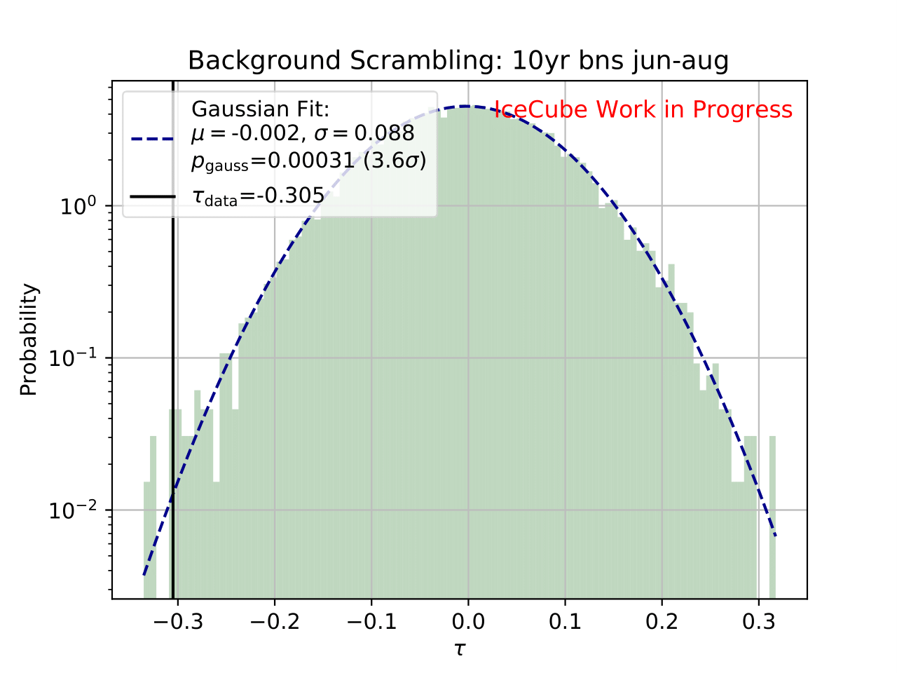
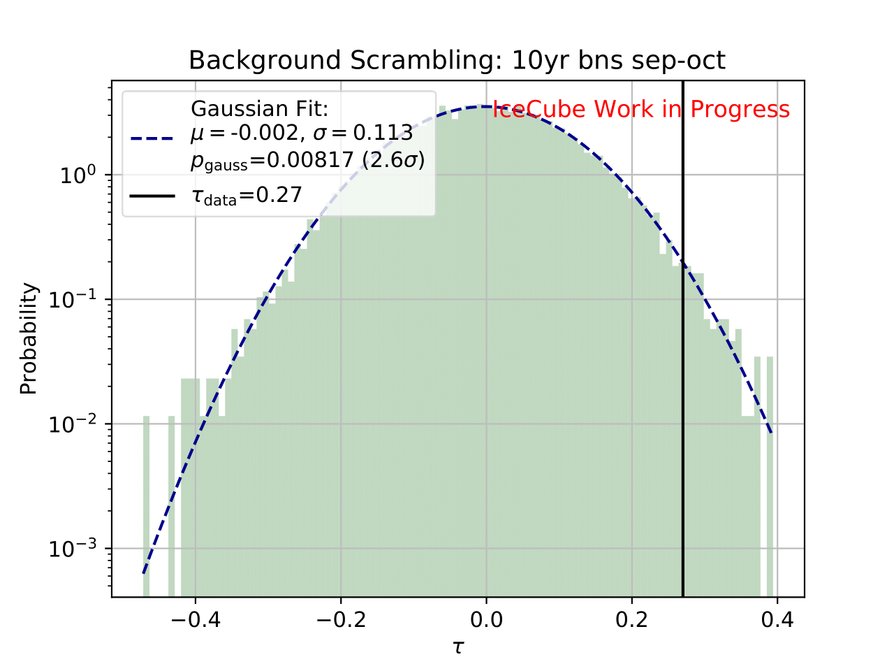
Even though a clear tendency towards an increased flux for the season from December to February is observable on the burn sample, it has to be ensured that this observation has not been caused randomly. To investigate the likelihood of observing the given deviation from the mean annual flux by chance, the following background scrambling method has been developed:

First a test statistic (TS) \(\tau = \sum_{i=1}^{10} \frac{flux_{\mathrm{season},i}}{flux_{\mathrm{year},i}} -1\) is defined to measure the deviation of the seasonal deviation from the annual mean flux in energy bin 1-10. Here, the underflow and overflow bins are neglected since events in these bins are out of interest for the analysis. However, the definition of these is necessary to account for smearing in the unfolding process.

Scrambled data sets are created in the following manner. A value, either 0 (the respective season) or 1 (any other season), is randomly assigned to each run. The fraction of both values is given by a weight that compares the livetime of the respective season divided by the livetime of the complete data set (here: burn sample), hence the livetime fraction of the season compared to the complete all season data set. The so-called scrambled data set, corresponding to all events labeled with 0, is unfolded. This procedure is repeated over 10 000 trials and the test statistic value of each one is calculated. The seasonal livetime weight ensures that a season contains on average a fraction of events similar to the real data set. Statistical uncertainties are not yet included in this test.

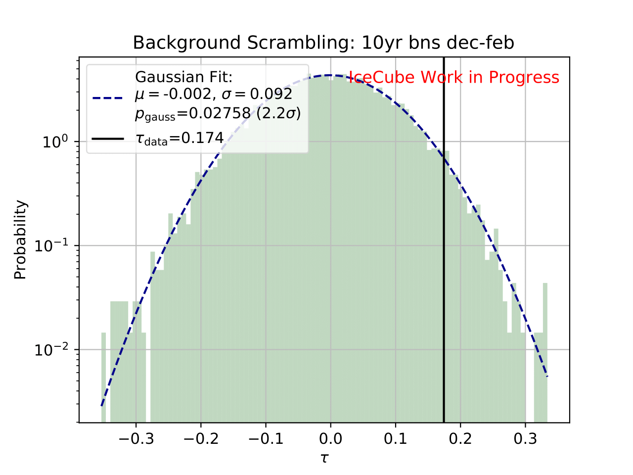
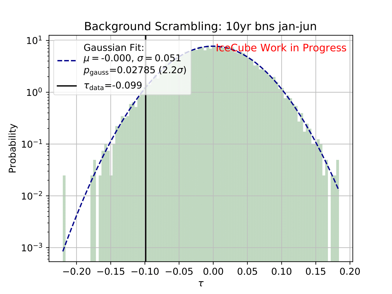
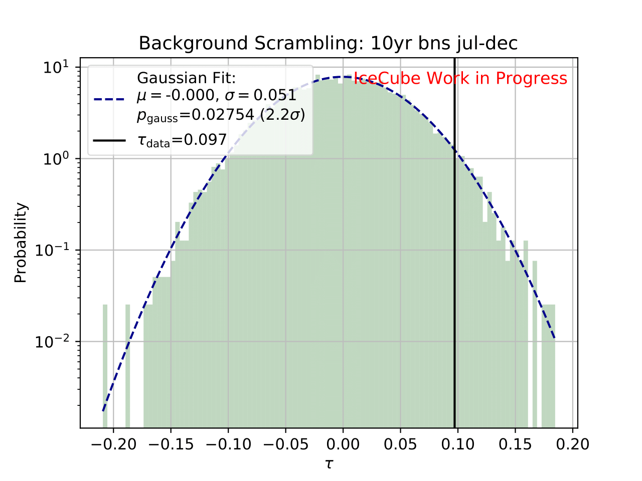
The distributions of the test statistic are displayed below. The p value and the corresponding significance of the unfolded result can be obtained by counting the more extreme values of the test statistic than the test statistic value obtained from the burn sample result (p value for data - black in figures below). 10 000 background trials, however, do not lead to an accurate p value which is desirably very small for a significant result. Hence, the p value can be obtained from a Gaussian distribution by the integration of the distribution’s tail. As illustrated below, the test statistic distributions are fitted with a Gaussian function. The p value from the Gaussian distribution is calculated by integrating the distribution tail above/below the critical test statistic value \(\tau_{crit}\). Since this is a one-sided p value, the right tail is integrated if \(\tau_{crit}>0\) and the left one if \(\tau_{crit}<0\). This assumption is valid since the test statistic is centered around 0. This is expected for a random scrambling which shouldn’t show any seasonal dependence.

Statistical uncertainties (as displayed in the ratio plots) are not respected in the significance calculation. The uncertainty is expected to be very small on the complete sample so that it is negligible for the complete data set.

Display of Gaussian fit in log-plot:

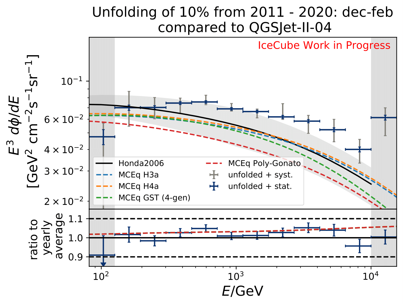
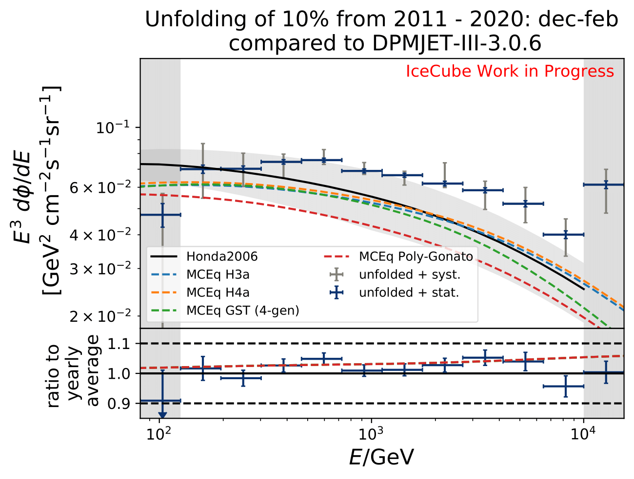
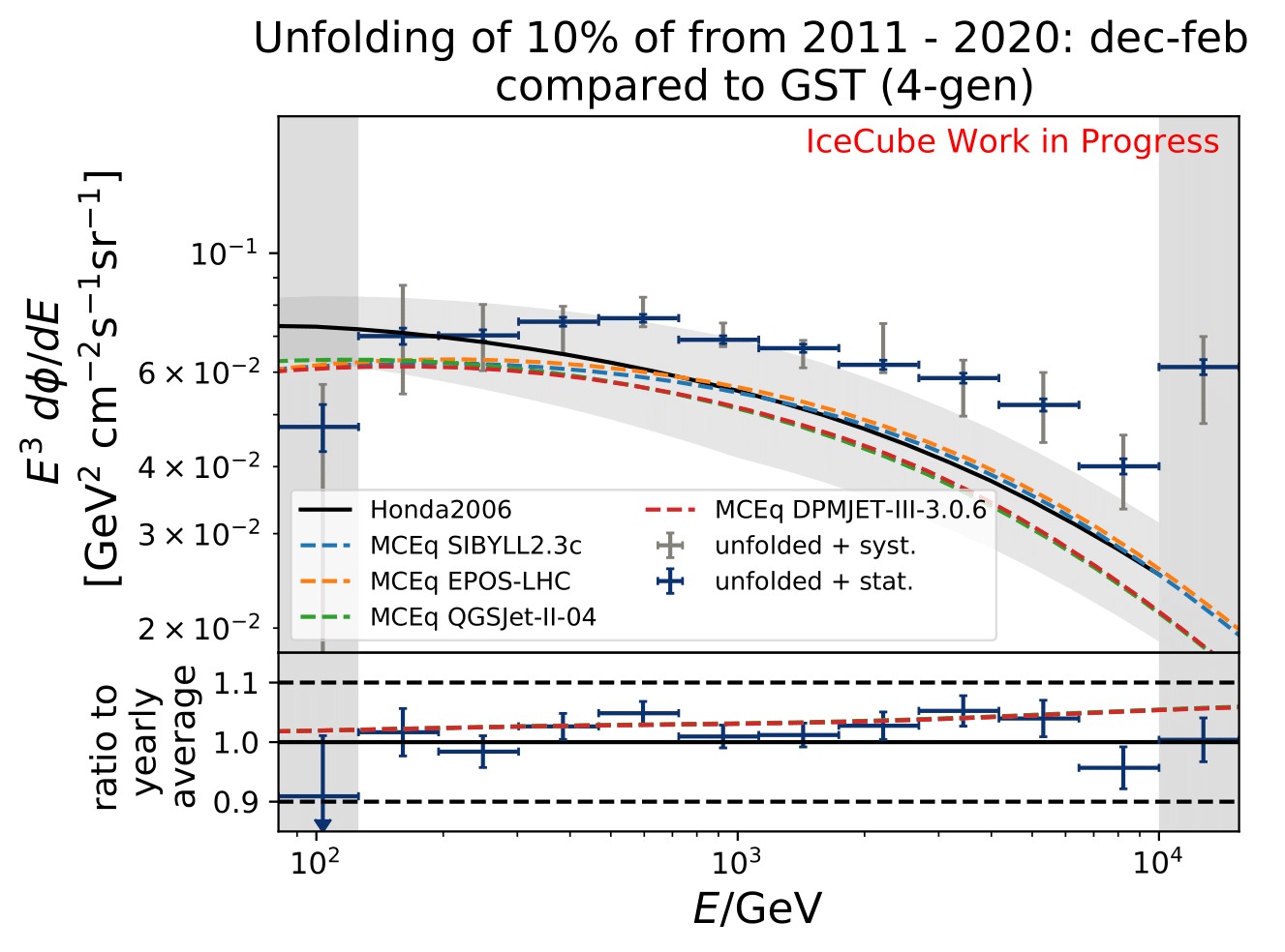
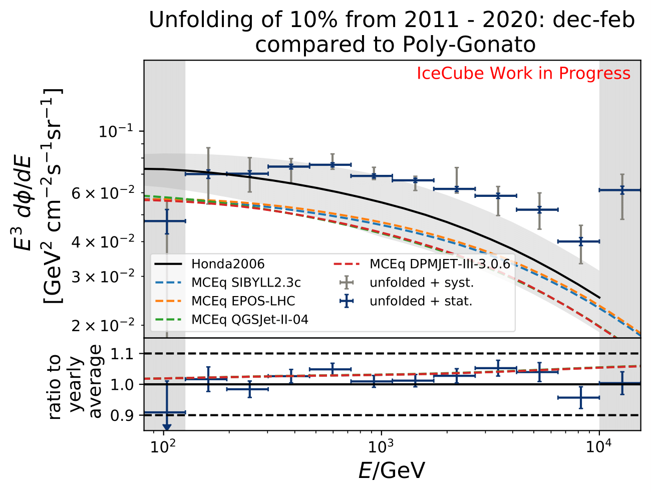
Comparison to MCEq

The software package MCEq calculates particle fluxes using different atmospheric and hadronic interaction models. This allows to predict seasonal variations on the atmospheric neutrino flux, which can be compared to the unfolding results. The atmospheric model MSIS00_IC is the NRLMSISE-00 global static atmospheric model from NASA centered to IceCube coordinates (so that the zenith angles are the same as in the IceCube data). Initially, the primary cosmic ray composition model H3a. The four implemented hadronic interaction models are selected with the latest version each. The muon neutrino flux (given in units of: \(GeV^{2} cm^{-2} s^{-1} sr^{-1}\)) is calculated for every month at six zenith angles between 90° and 120°. The zenith bins are created in terms of \(cos(\Theta)\). The monthly fluxes in each zenith bin are averaged over the whole zenith range and then averaged to construct seasonal flux predictions. The corresponding spectra are displayed below for every unfolded seasonal neutrino flux. No flux uncertainties are incorporated in the MCEq calculation. The unfolded burn sample spectrum for December-February is exemplarily compared to the seasonal flux predictions by MCEq. One model, either CR composition or hadronic interaction model is held constant, whereas the other models are varied. Four model are displayed at a time to be able to distinguish between the curves.

Proposal: Extension to 12yrs of data

The number of events is extrapolated adding an additional 42 000 events per year. This is obtained from the burn sample estimate (10% from 2011 to 2020) because the burn sample of this analysis corresponds approx. to one year of experimental data.

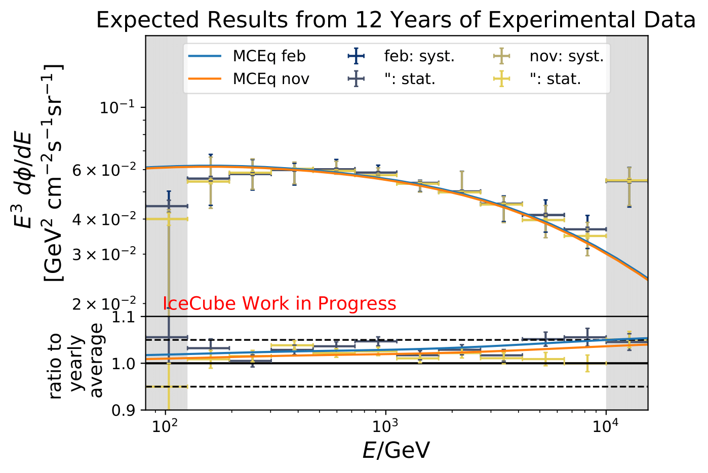
The uncertainty of the flux ratio shrink by 2-9% depending on energy bin and season.