Unblinding Results¶

The unblinded results will be displayed in this section. The use of the complete data set from 2011 (IC86) to 2022 has been approved. The complete data sample contains 523736 events within 11.5 years of data.

Monthly spectra will be unfolded and its deviation from the annual average flux. The variation strength will be fitted per month and each energy bin. The results will be compared to predictions from MCEq and the spectral index deviation from the annual average flux will be determined. Annual unfolding will be performed to provide consistency between the years.

Monthly Neutrino Rate¶

In order to determine where the mismatch between unfolding and MCEq comes from in particular months, the neutrino rate is shown for each month in the 12yr data sample.

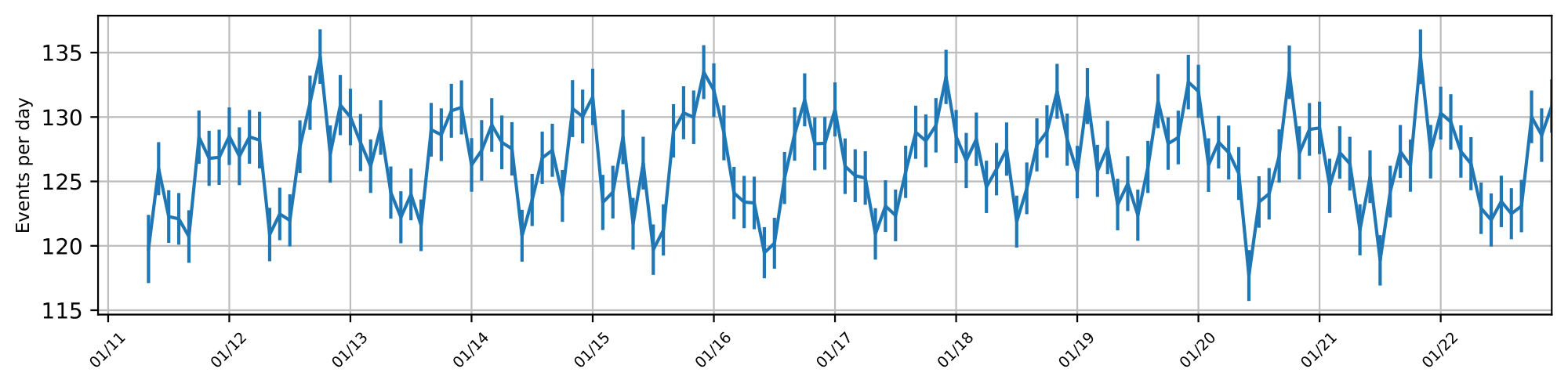
The first months of 2011 show a lower rate than the other years. This is likely to originate from the uncompleted detector setup. The current IC-86 string configuration was completed at the end of 2010, but the run start including new detector setups is switching in May for each year. This means that the additional seven strings are only included in the reconstruction from May onward, which results in a lower rate for the respective month. Same behavior is observable below, where single years have been unfolded as post-unblinding crosschecks. Hence, the analysis is shifted to 11.5 years of data starting from May 7, 2011.

Unfolded 11.5yr Spectra/Unfolded Ratios¶

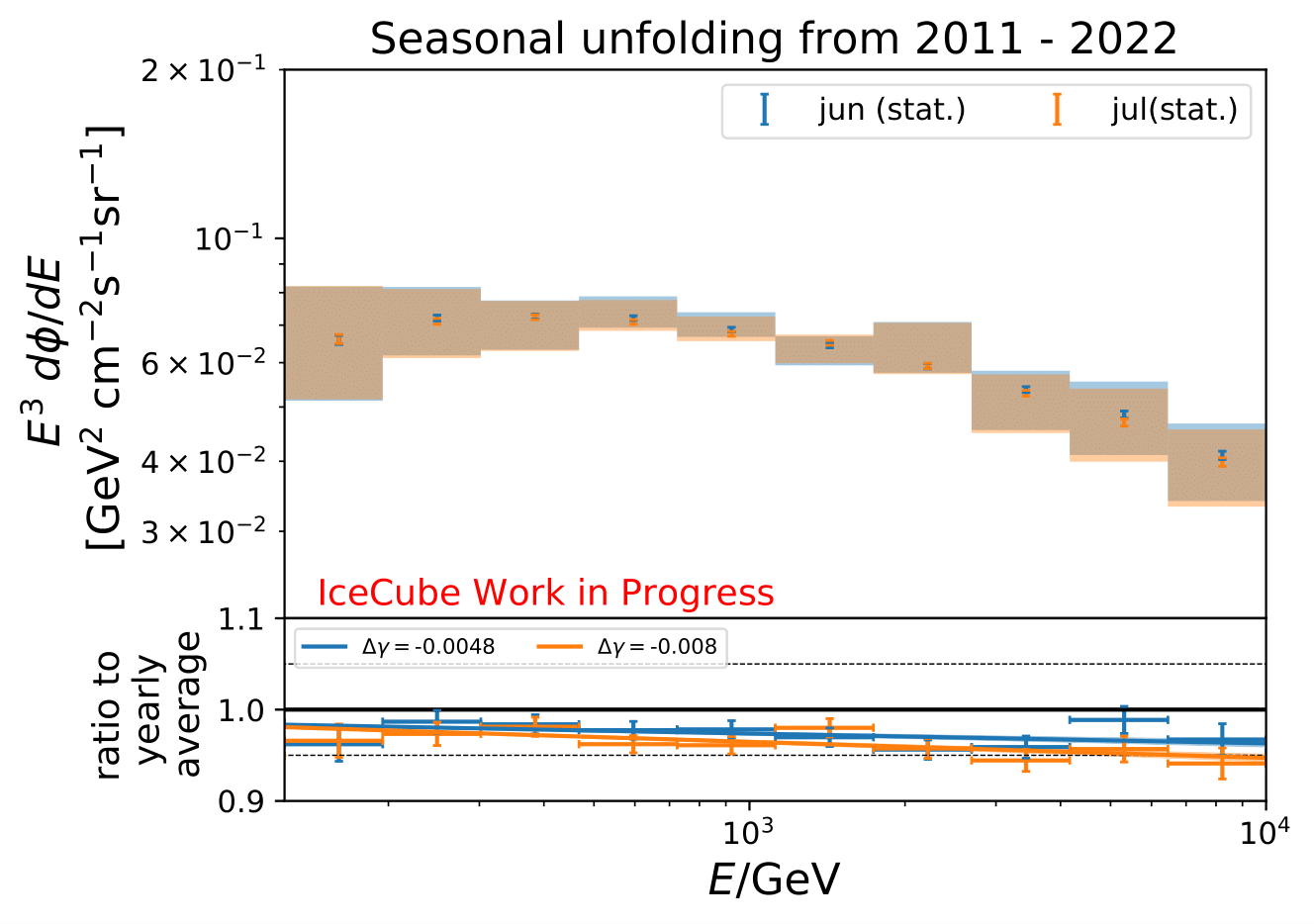
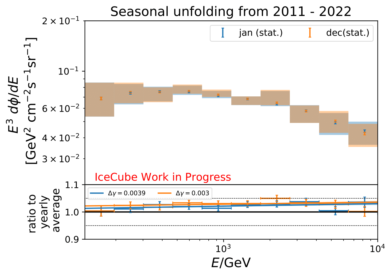
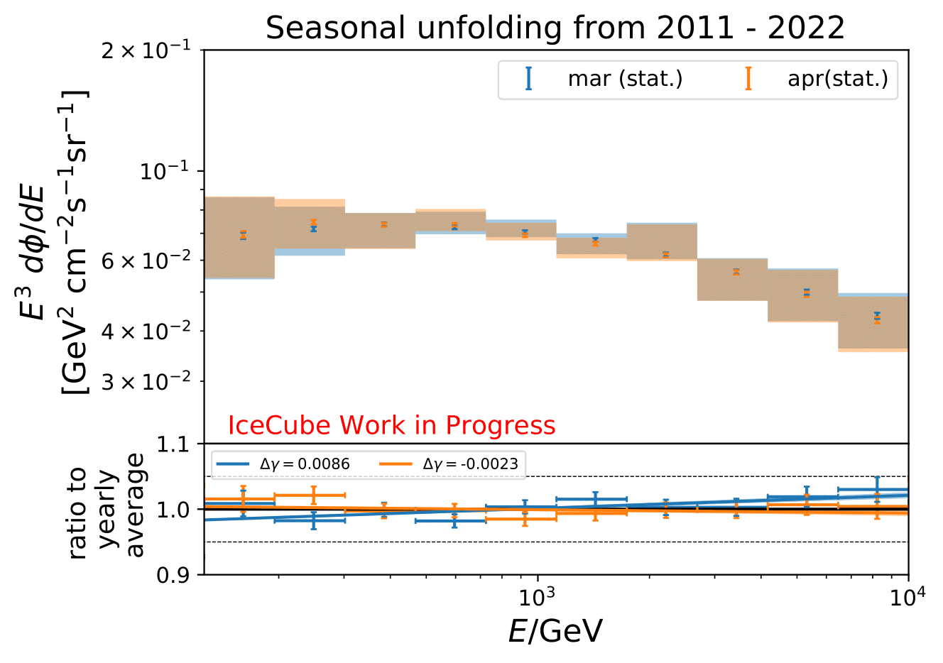
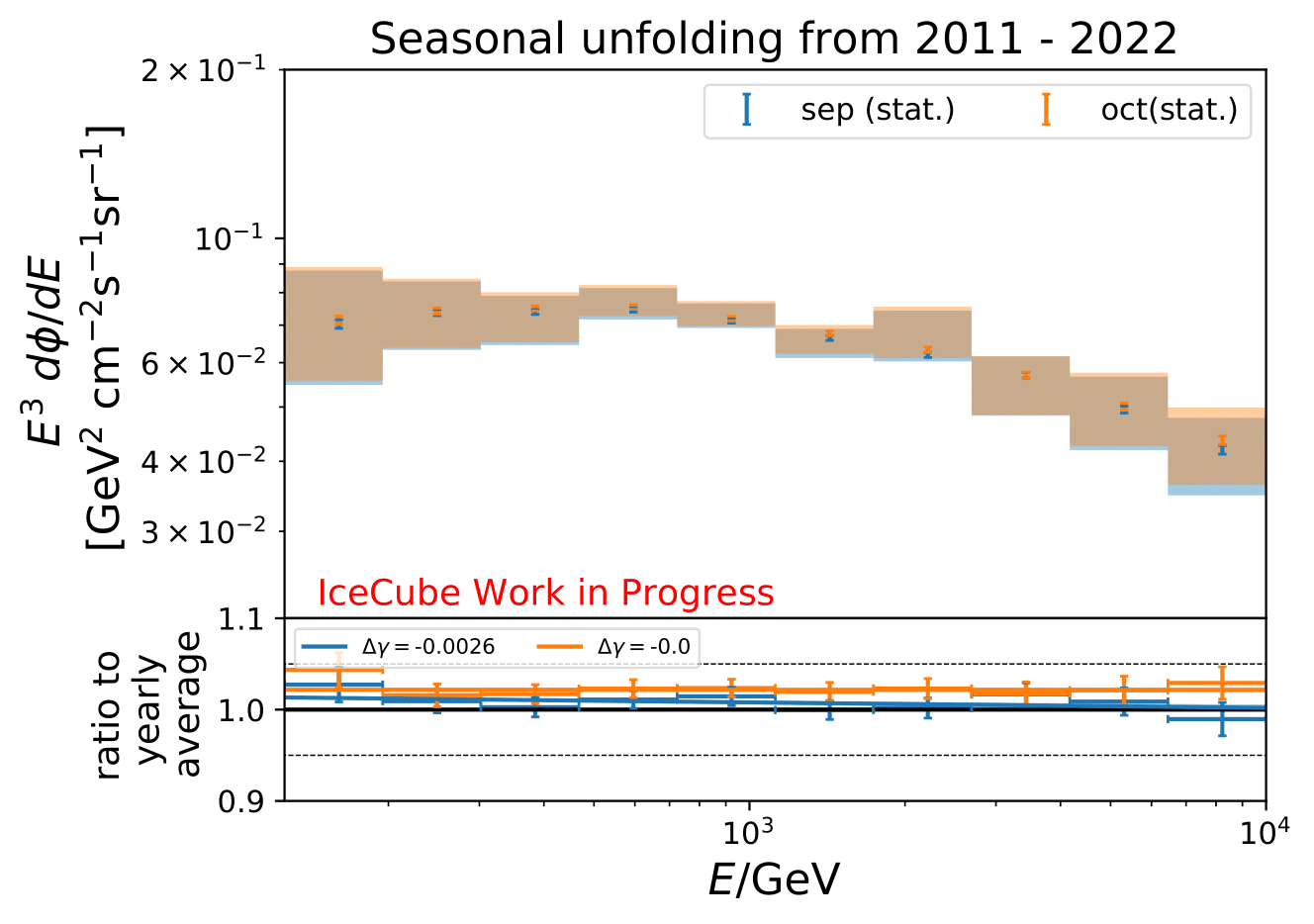
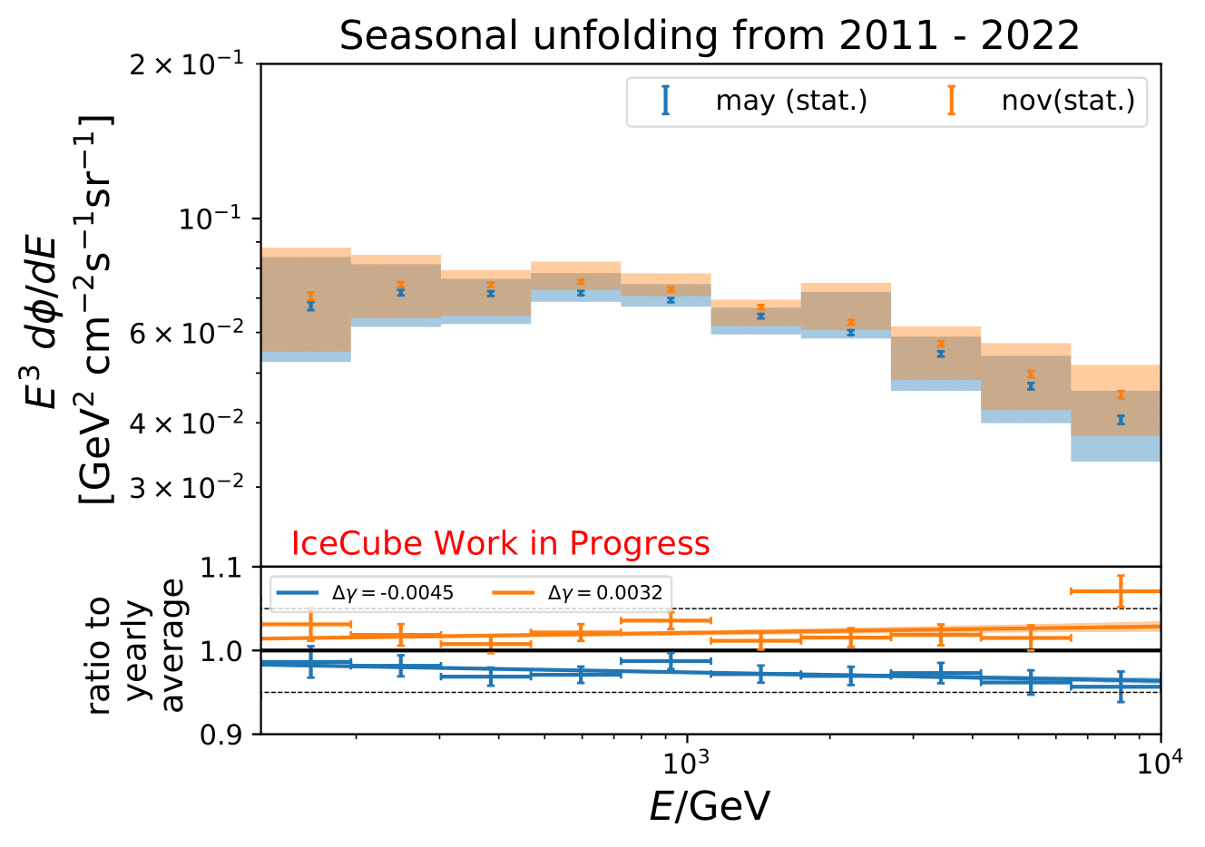
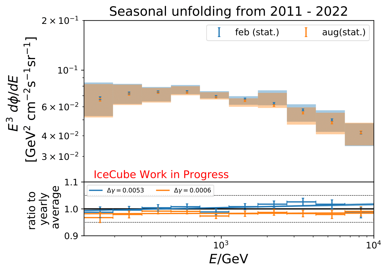
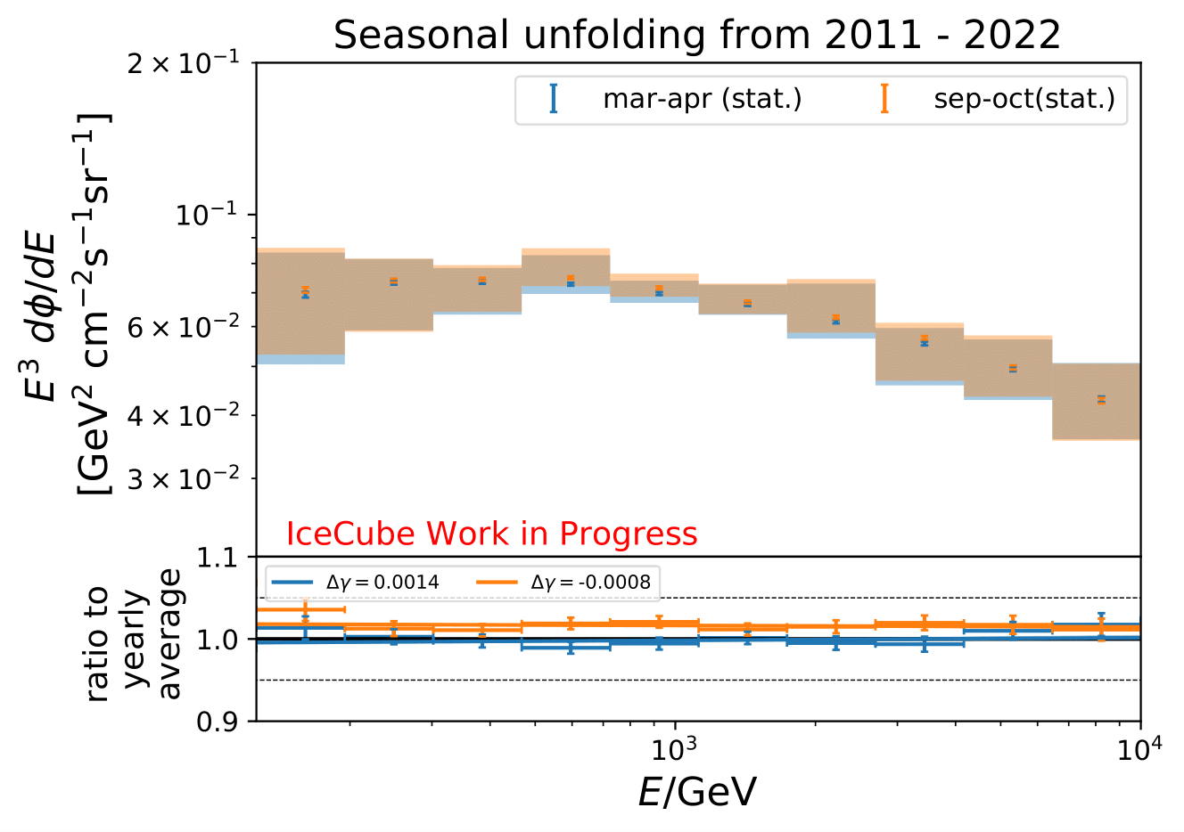
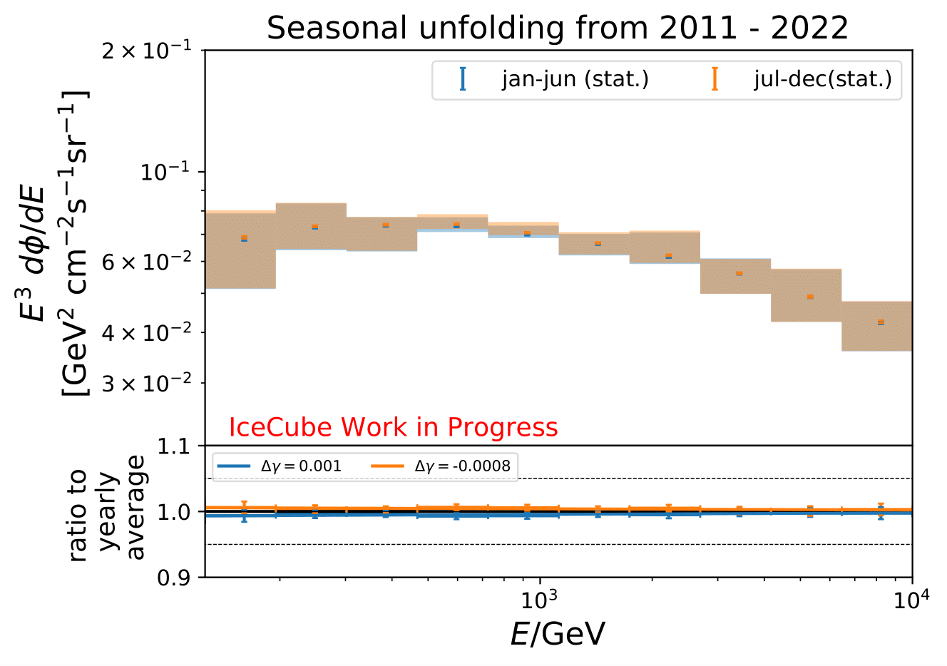
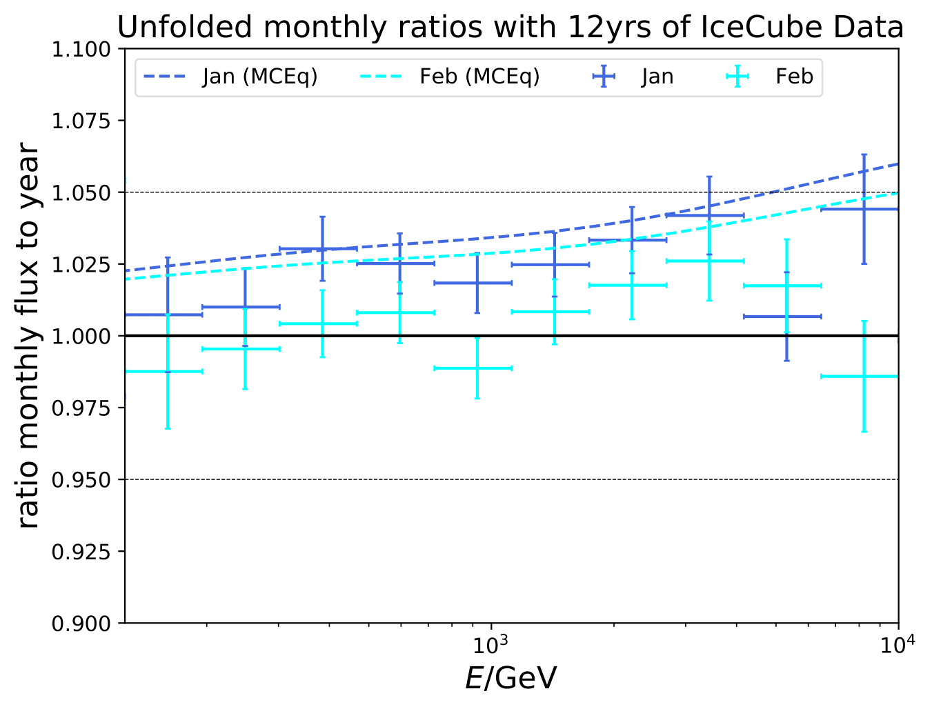
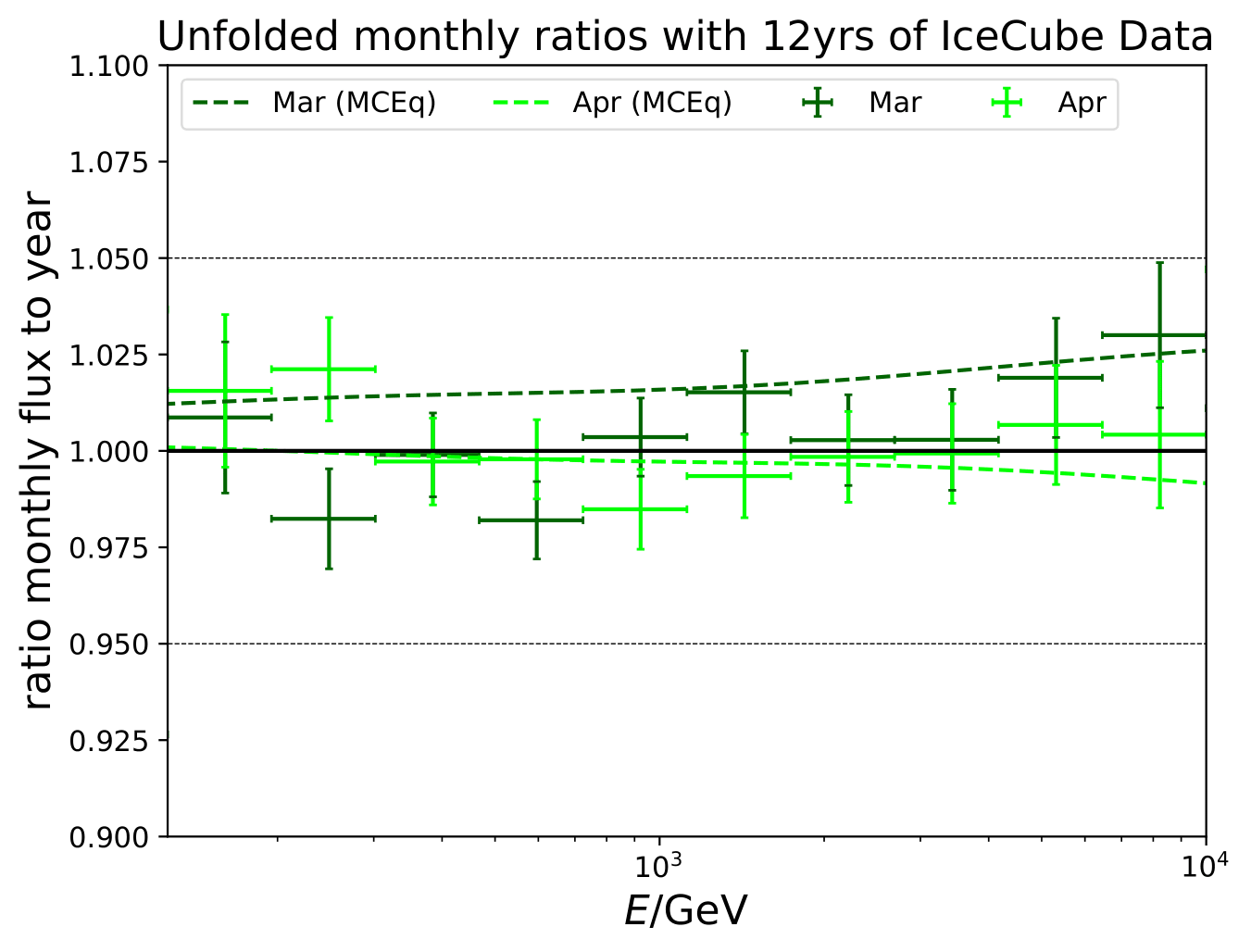
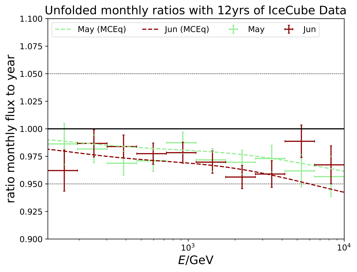
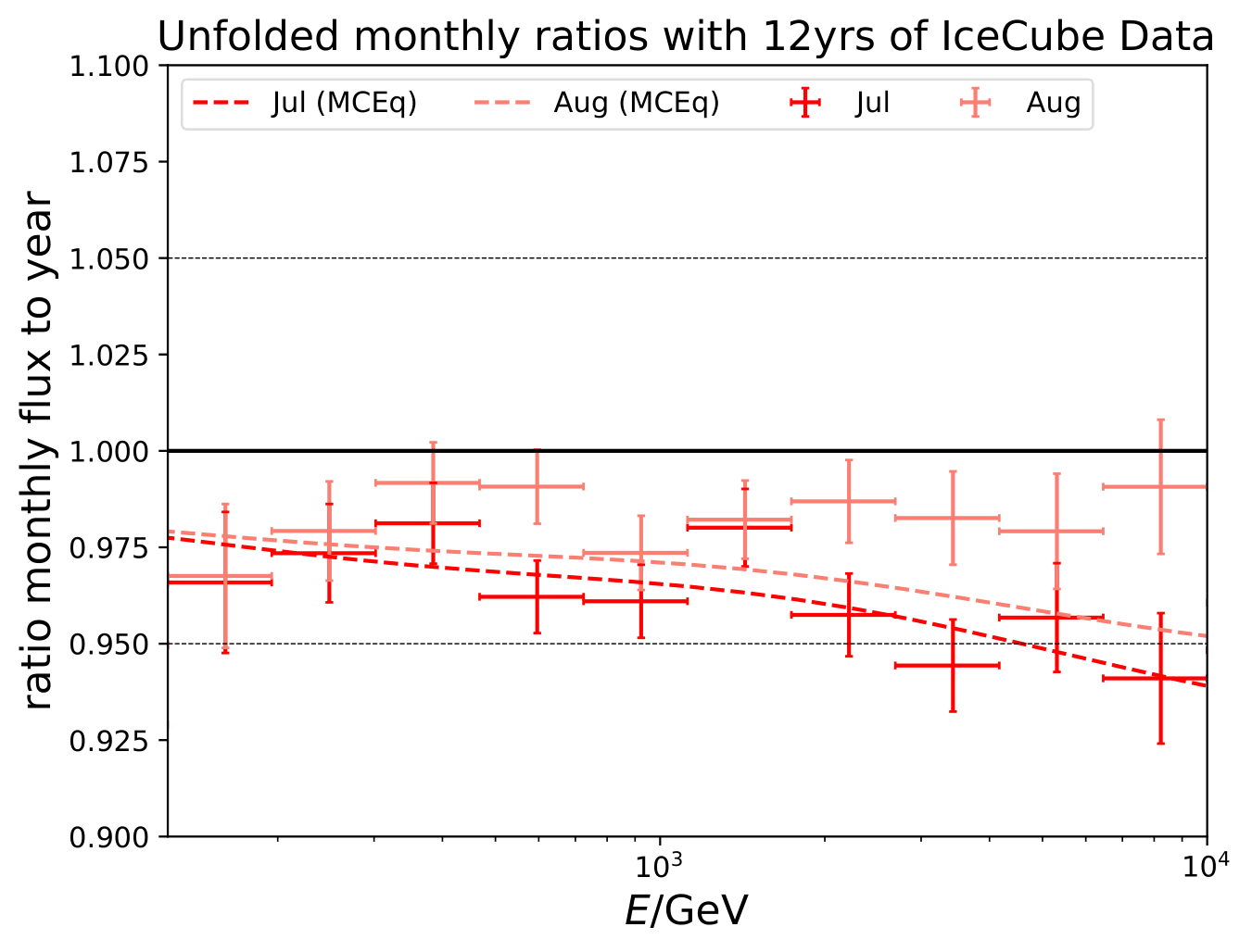
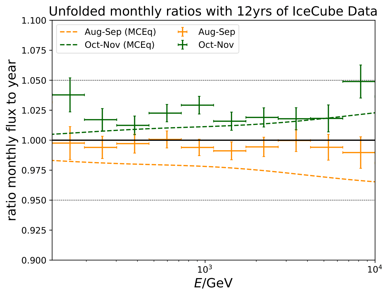
Shaded areas in the unfolded spectrum display systematic uncertainties. Statistical uncertainties are displayed by caps in the error bars. A fit of spectral index shift is performed on the ratio of seasonal flux to annual average flux. MCEq predictions are denoted as dashed lines.

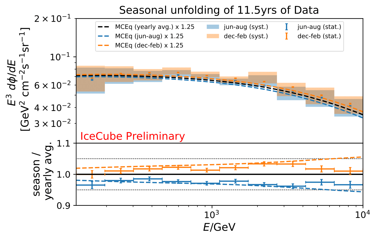
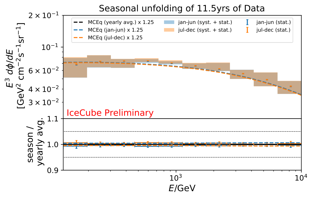
../_images/unblinded_e3_12yr_jun-aug_dec-feb_sys_90-120_ratio_cblind-1.png

../_images/unblinded_e3_12yr_jan-jun_jul-dec_sys_90-120_ratio_cblind-1.png

The significance is determined in a \(\chi^2\)-test with respect to statistical uncertainties of the ratio. The deviation of the total seasonal spectral ratio to the annual average is quantified.

Significance per Season¶
Season	Significance / \(\sigma\)
jun-aug	10.4
dec-feb	7.0
jan-jun	0.3
jul-dec	0.2
may-aug	15.9
oct-jan	12.3
jan	4.6
feb	0.7
mar	0.8
apr	0.2
may	5.3
jun	5.7
jul	8.5
aug	2.4
sep	0.4
oct	3.7
nov	4.4
dec	5.6

With spectral index shift fit:

../_images/unblinded_e3_12yr_jun_jul_90-120_ratio_fit-1.png

../_images/unblinded_e3_12yr_jan_dec_90-120_ratio_fit-1.png

../_images/unblinded_e3_12yr_mar_apr_90-120_ratio_fit-1.png

../_images/unblinded_e3_12yr_sep_oct_90-120_ratio_fit-1.png

../_images/unblinded_e3_12yr_may_nov_90-120_ratio_fit-1.png

../_images/unblinded_e3_12yr_feb_aug_90-120_ratio_fit-1.png

../_images/unblinded_e3_12yr_mar-apr_sep-oct_90-120_ratio_fit-1.png

../_images/unblinded_e3_12yr_jan-jun_jul-dec_90-120_ratio_fit-1.png

Comparison to MCEq:

../_images/monthly_ratio_unblind_withmceq_jan_feb-1.png

../_images/monthly_ratio_unblind_withmceq_mar_apr-1.png

../_images/monthly_ratio_unblind_withmceq_may_jun-1.png

../_images/monthly_ratio_unblind_withmceq_jul_aug-1.png

../_images/monthly_ratio_unblind_withmceq_sep_oct-1.png

../_images/monthly_ratio_unblind_withmceq_nov_dec-1.png

../_images/monthly_ratio_unblind_withmceq_dec-jan_jun-jul-1.png

../_images/monthly_ratio_unblind_withmceq_feb-mar_apr-may-1.png

../_images/monthly_ratio_unblind_withmceq_aug-sep_oct-nov-1.png

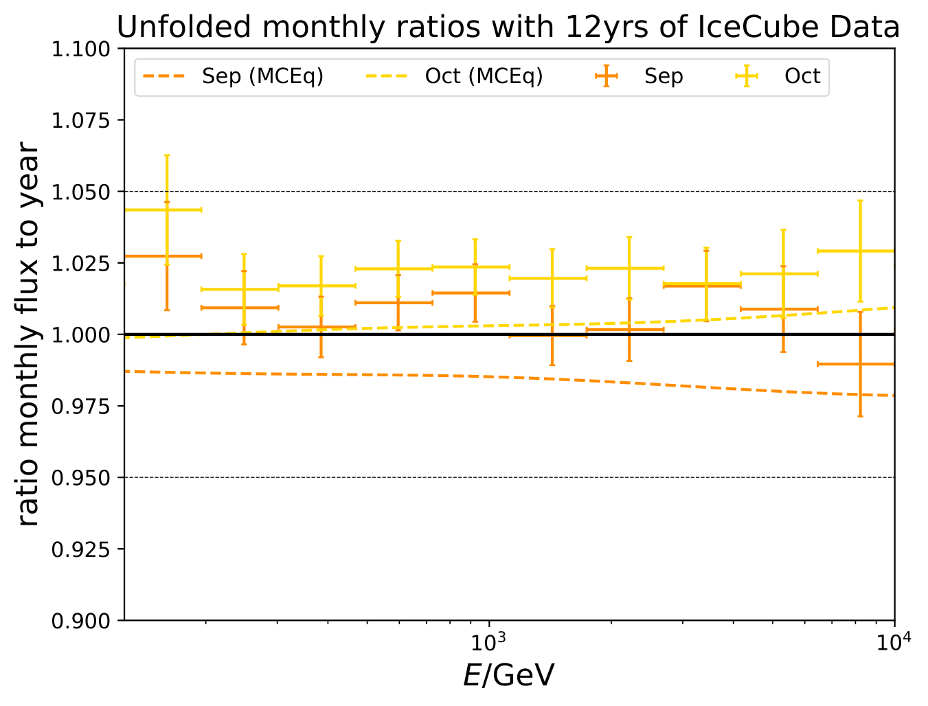
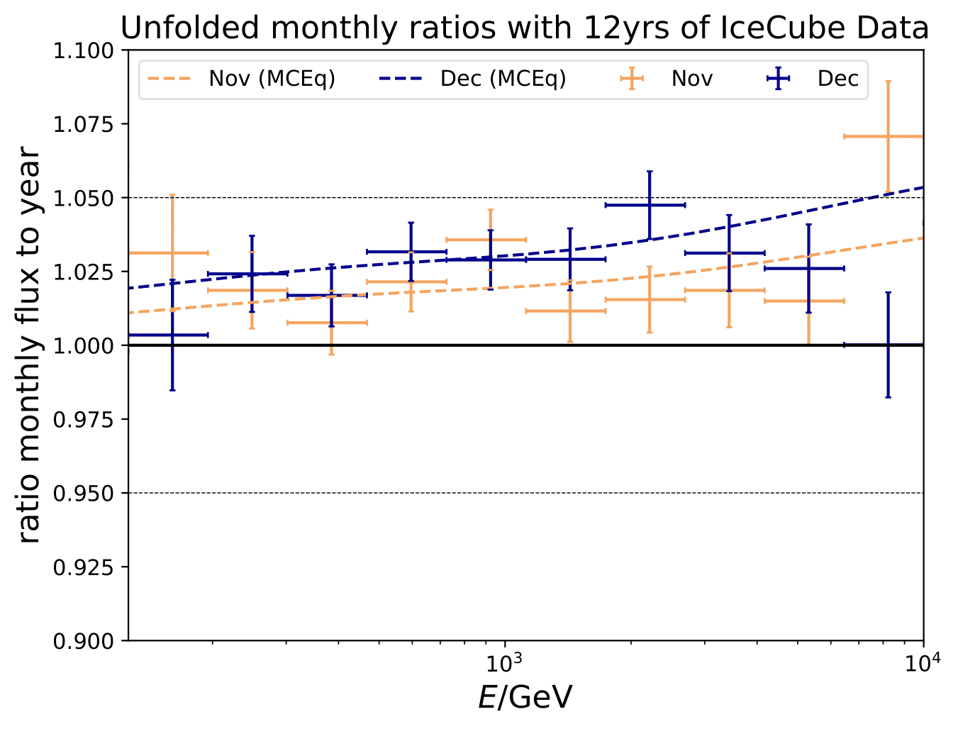
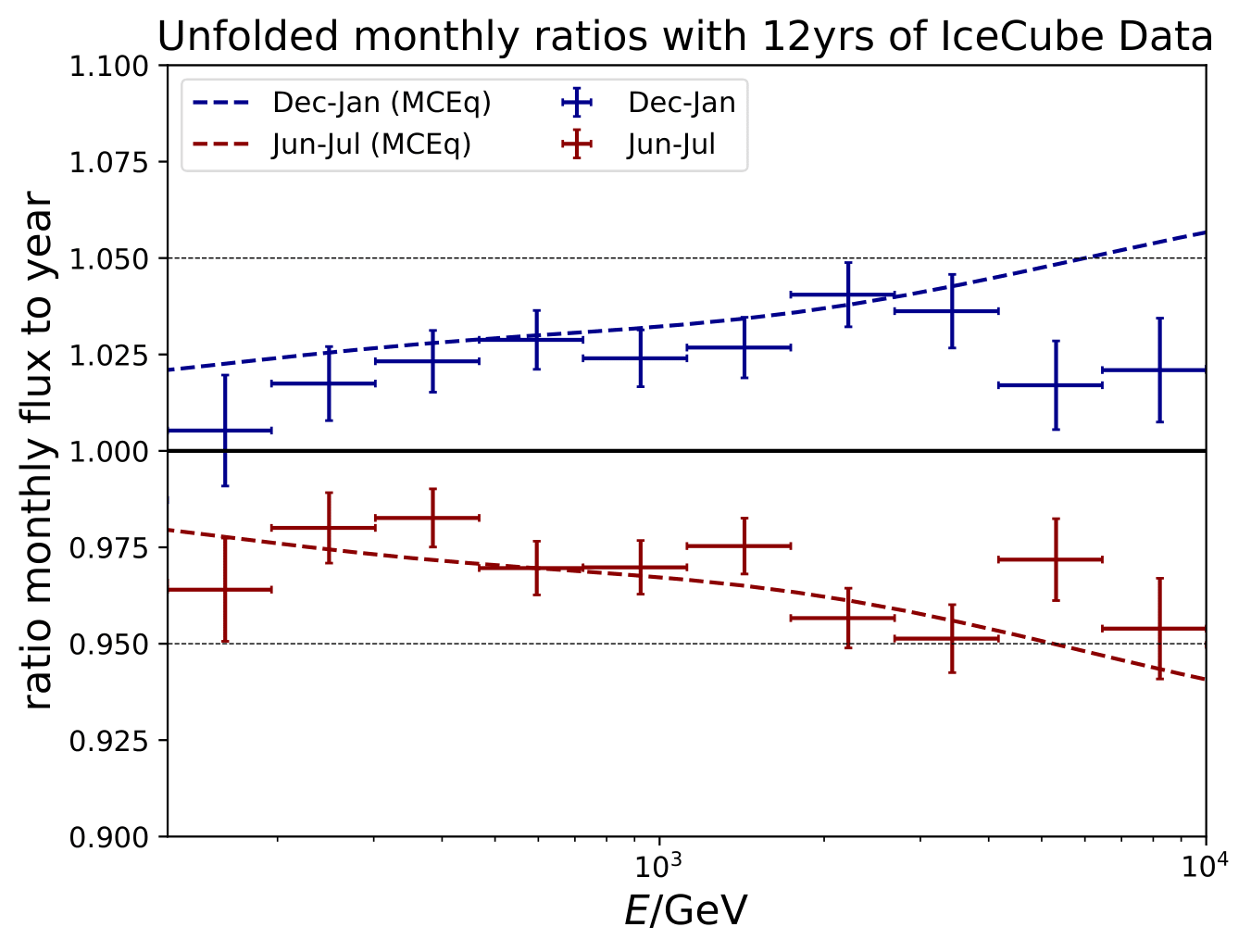
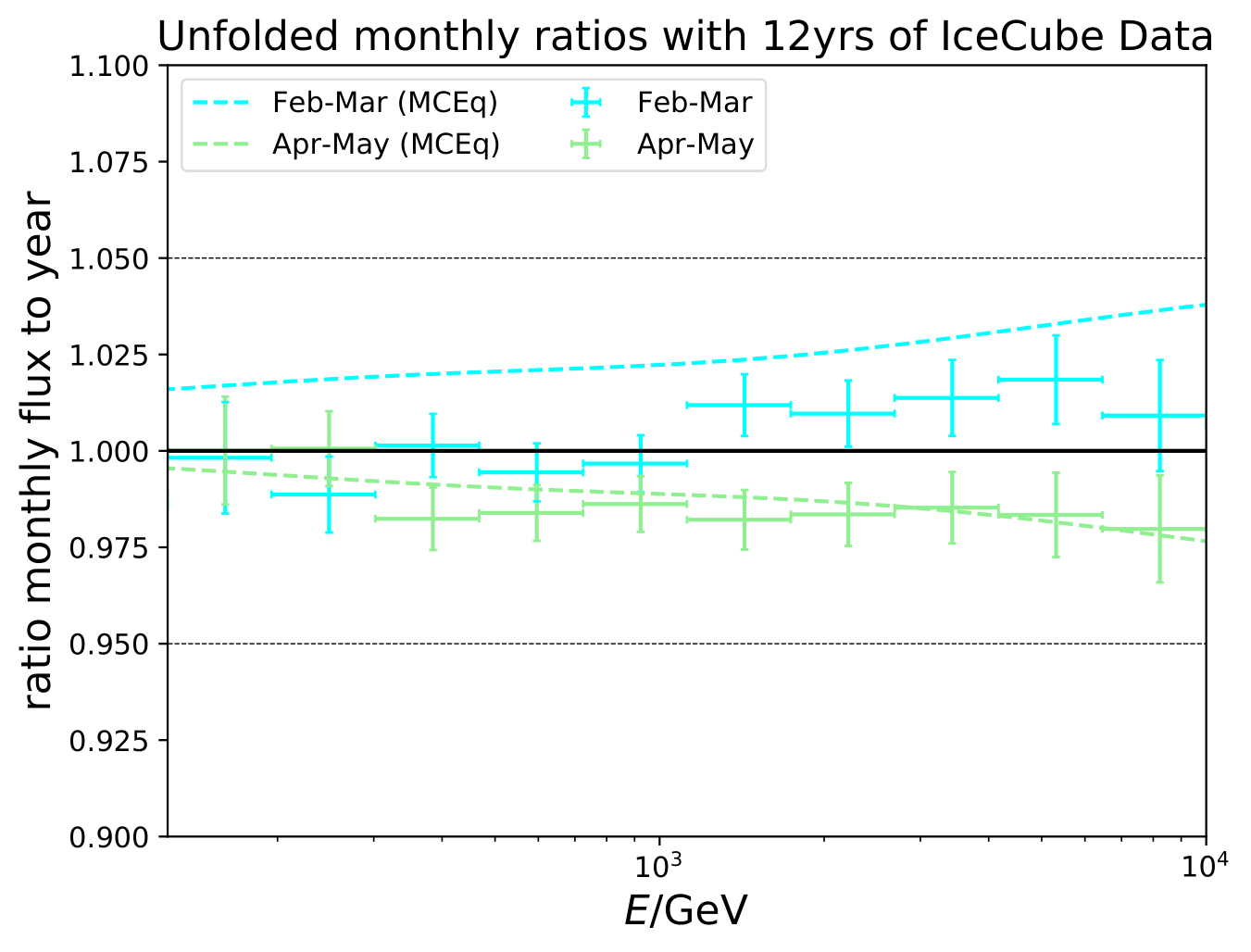
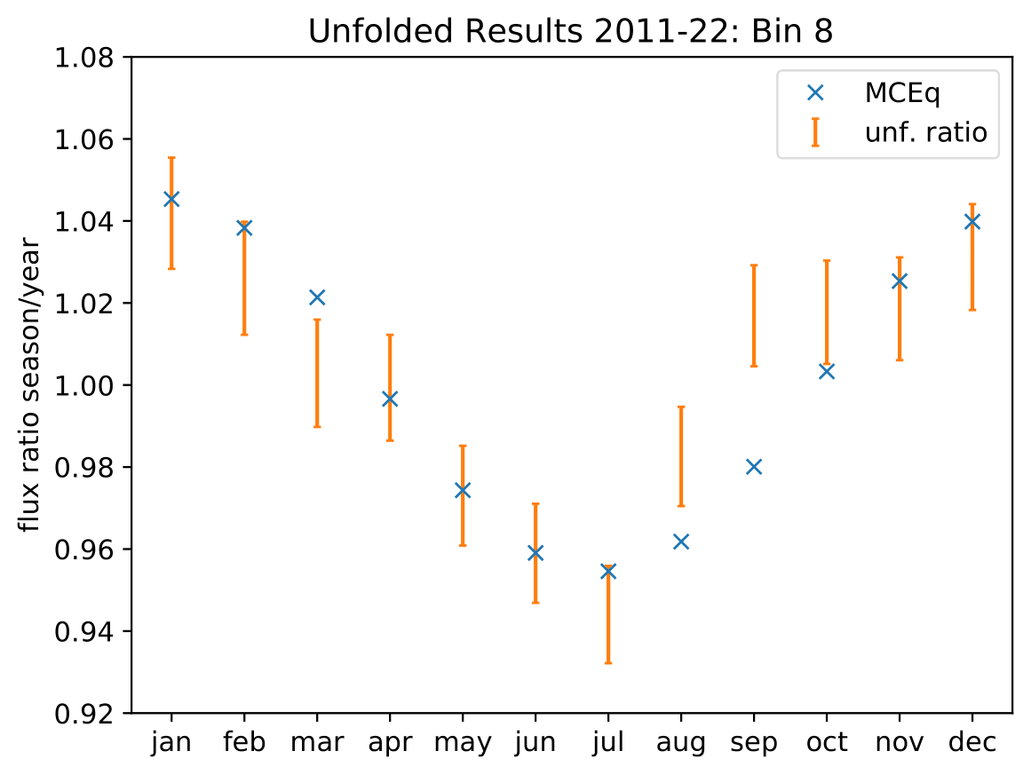
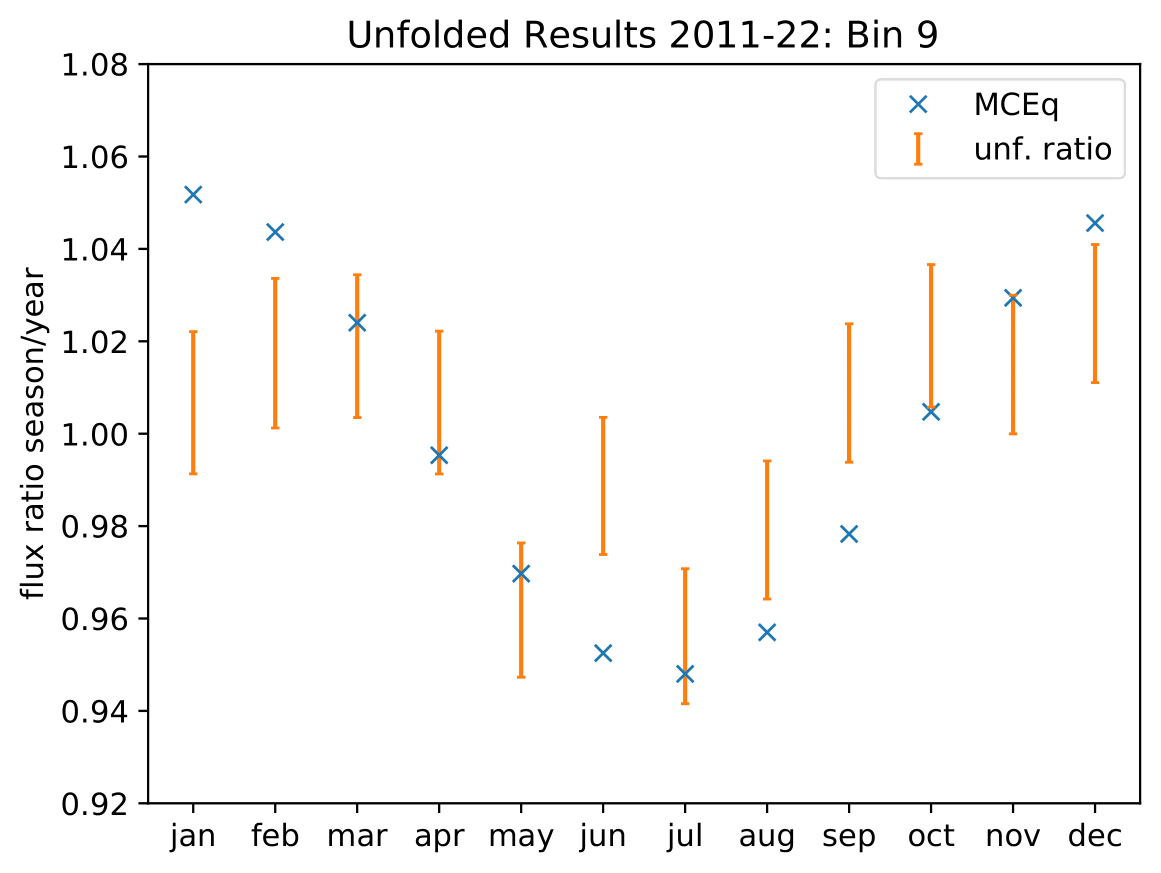
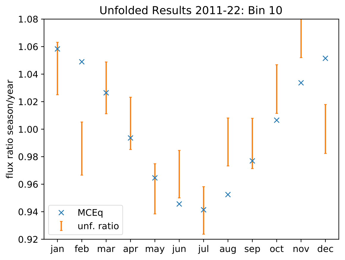
Comparison of Unfolded Ratio to MCEq¶

The unfolded ratios of seasonal to annual average flux are compared to predicted ratios by MCEq. This test has been performed on pseudo-data unfolding and can be found in the QA section. The MCEq flux is calculated at the bin midth using the spline fits from the MCEq weighting. No uncertainty is considered on the MCEq prediction, the statistical uncertainty is propagated to the ratio. A linear fit is performed to determine whether both, the unfolded ratio and MCEq predictions, are compatible. A \(\chi^2\)-test indicates whether the unfolded result is represented by the MCEq prediction. The nullhypothesis of the unfolded result not following the MCEq prediction is only ruled out by very small p-values. High p-values indicate that the nullhypothesis cannot be rejected to high significance.

../_images/ratio_mcequnfolding_unblind_mean_jan_mceqtheoryflux_withuncertaintyinfit-1.png

../_images/ratio_mcequnfolding_unblind_mean_feb_mceqtheoryflux_withuncertaintyinfit-1.png

../_images/ratio_mcequnfolding_unblind_mean_mar_mceqtheoryflux_withuncertaintyinfit-1.png

../_images/ratio_mcequnfolding_unblind_mean_apr_mceqtheoryflux_withuncertaintyinfit-1.png

../_images/ratio_mcequnfolding_unblind_mean_may_mceqtheoryflux_withuncertaintyinfit-1.png

../_images/ratio_mcequnfolding_unblind_mean_jun_mceqtheoryflux_withuncertaintyinfit-1.png

../_images/ratio_mcequnfolding_unblind_mean_jul_mceqtheoryflux_withuncertaintyinfit-1.png

../_images/ratio_mcequnfolding_unblind_mean_aug_mceqtheoryflux_withuncertaintyinfit-1.png

../_images/ratio_mcequnfolding_unblind_mean_sep_mceqtheoryflux_withuncertaintyinfit-1.png

../_images/ratio_mcequnfolding_unblind_mean_oct_mceqtheoryflux_withuncertaintyinfit-1.png

../_images/ratio_mcequnfolding_unblind_mean_nov_mceqtheoryflux_withuncertaintyinfit-1.png

../_images/ratio_mcequnfolding_unblind_mean_dec_mceqtheoryflux_withuncertaintyinfit-1.png

../_images/ratio_mcequnfolding_unblind_mean_dec-feb_mceqtheoryflux_withuncertaintyinfit-1.png

../_images/ratio_mcequnfolding_unblind_mean_jun-aug_mceqtheoryflux_withuncertaintyinfit-1.png

../_images/ratio_mcequnfolding_unblind_mean_jan-jun_mceqtheoryflux_withuncertaintyinfit-1.png

../_images/ratio_mcequnfolding_unblind_mean_jul-dec_mceqtheoryflux_withuncertaintyinfit-1.png

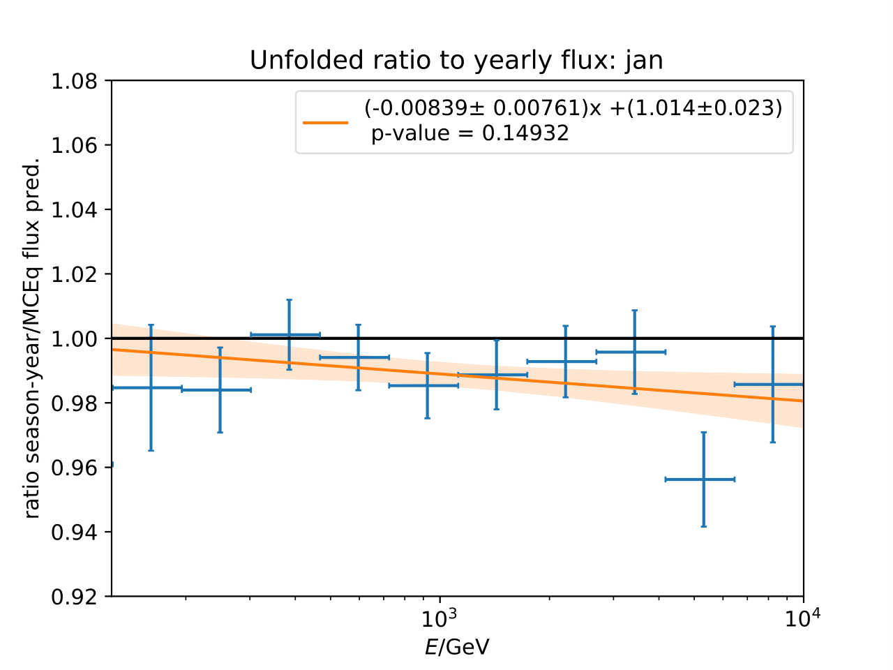
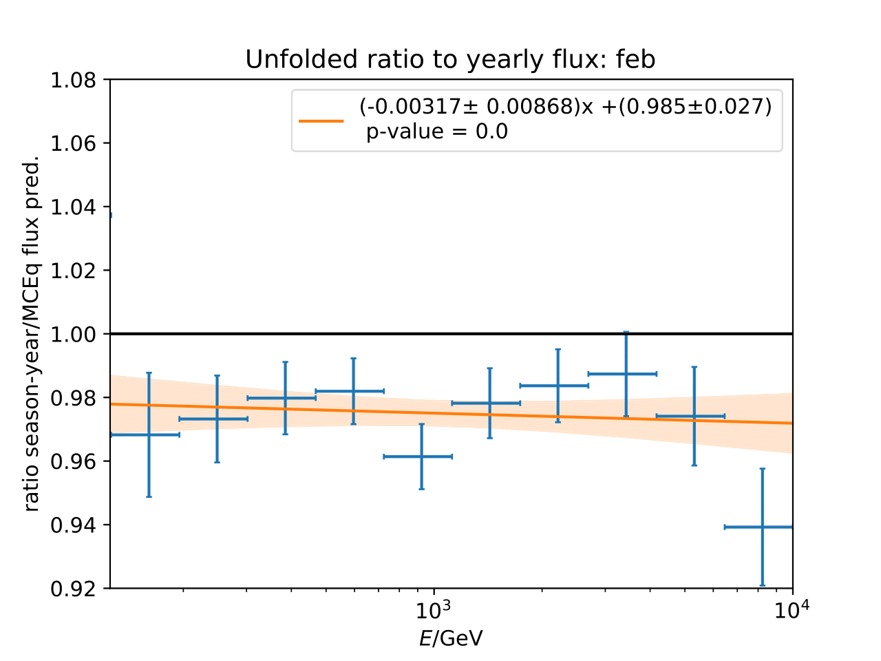
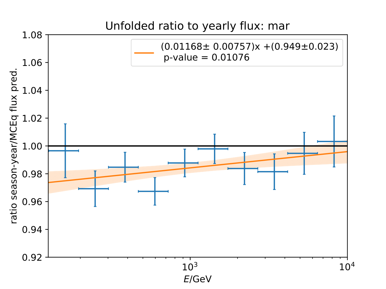
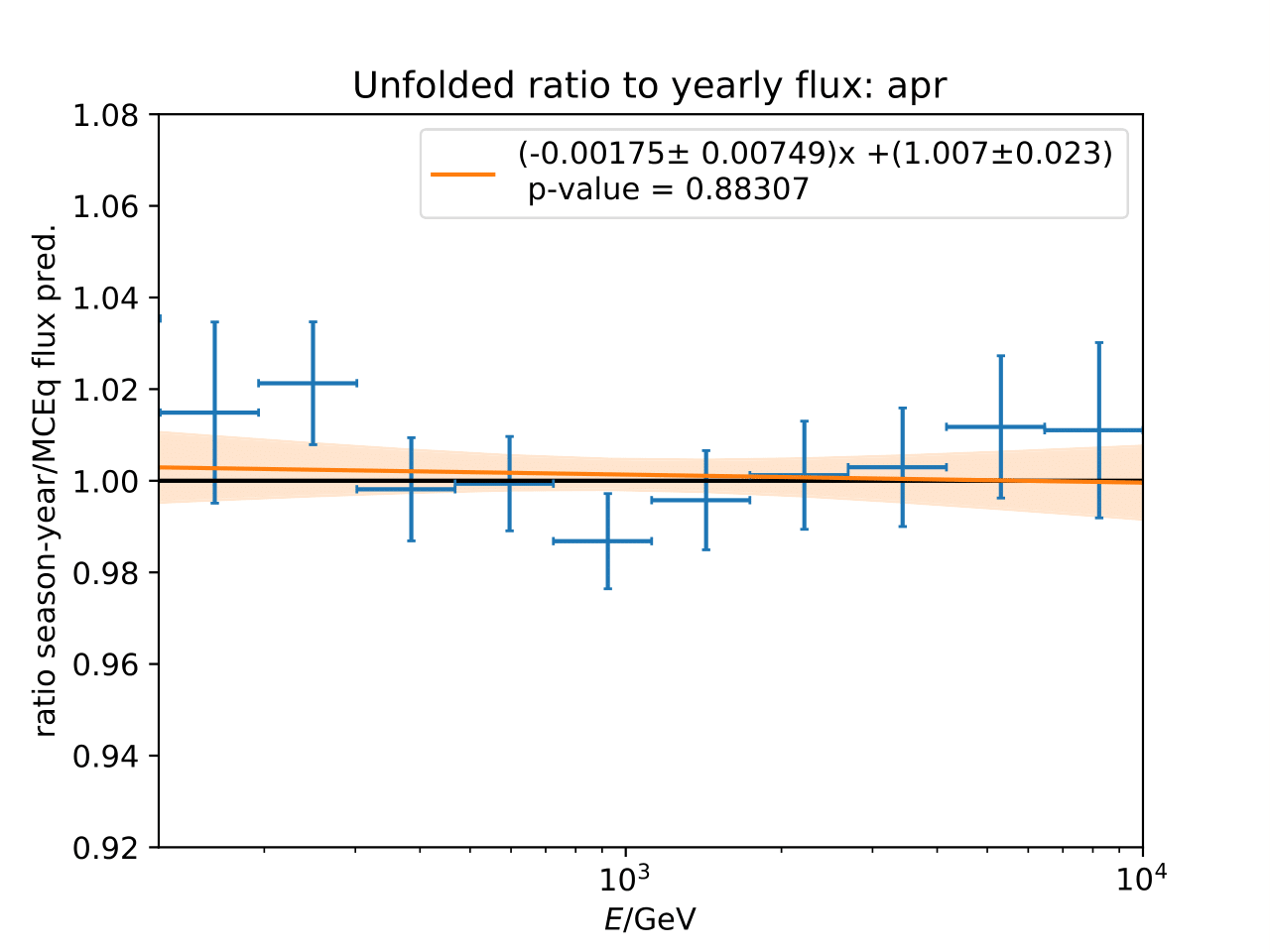
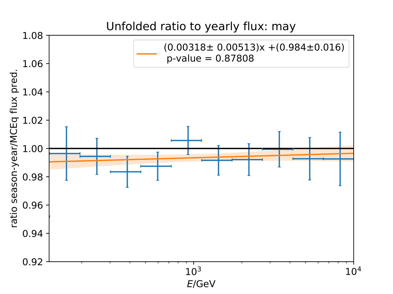
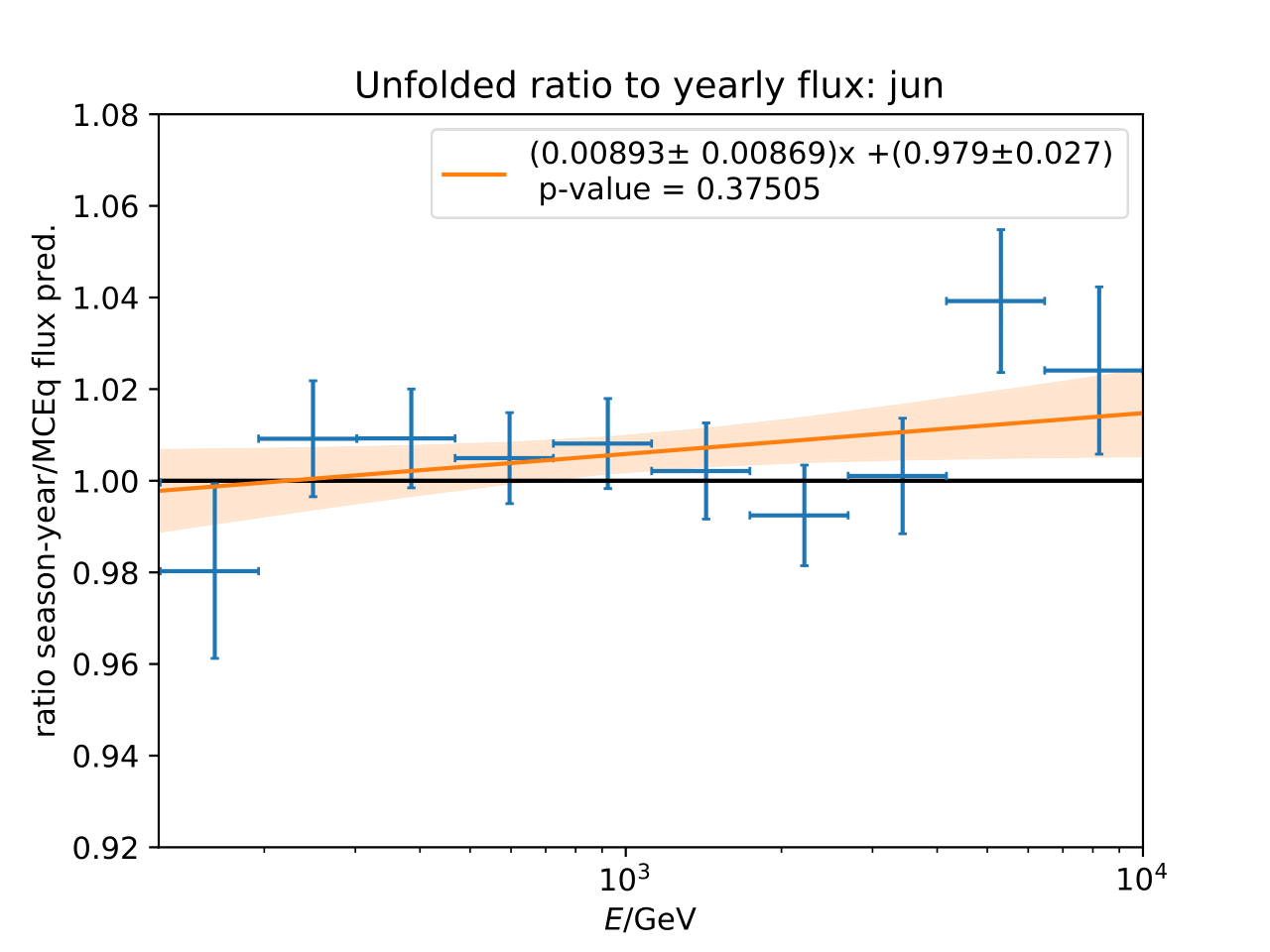
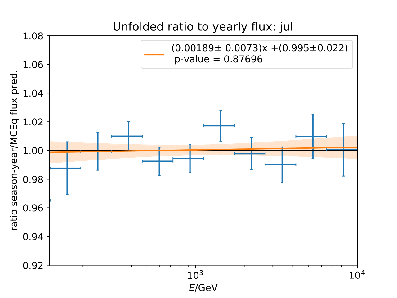
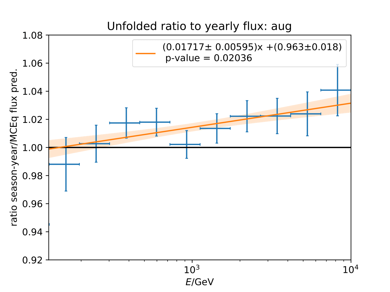
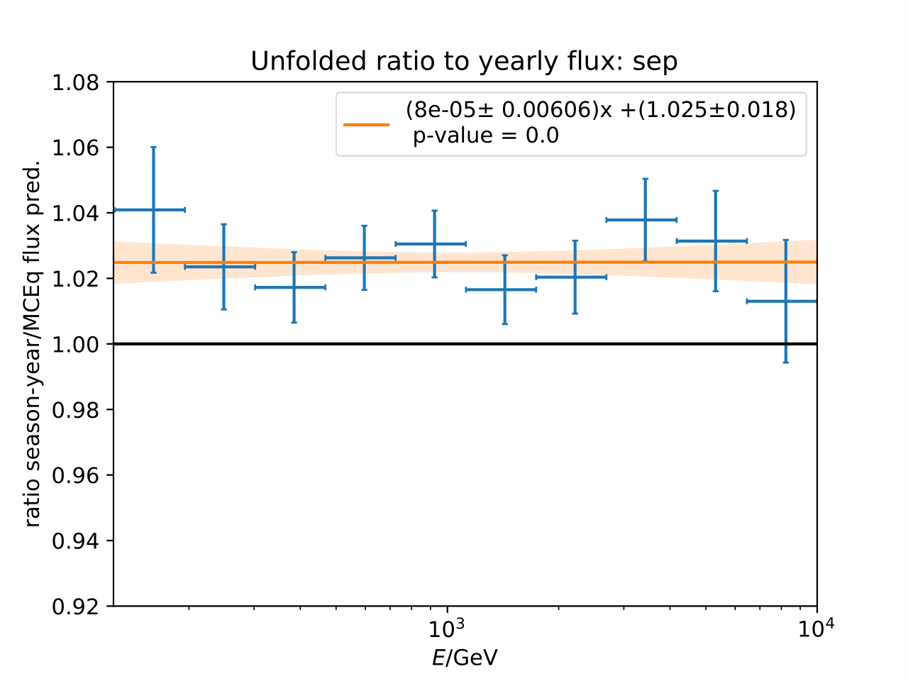
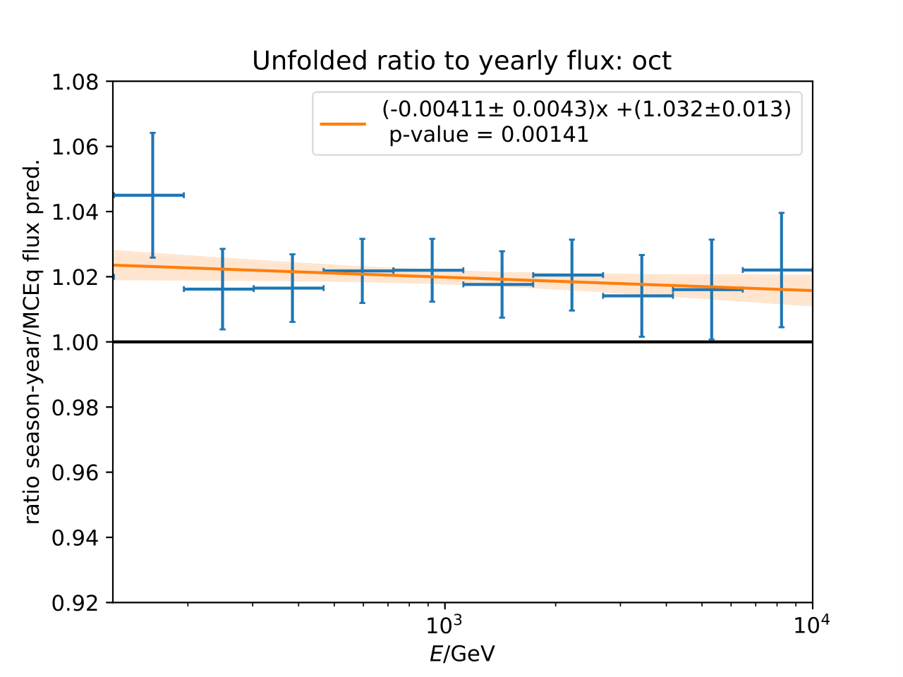
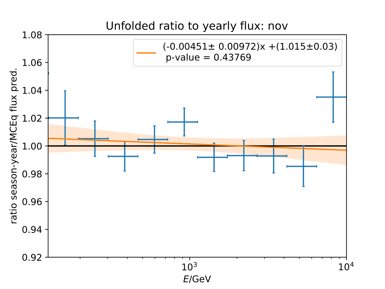
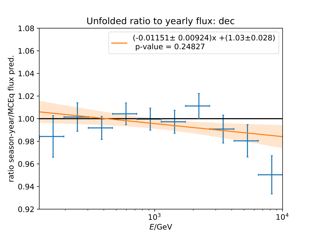
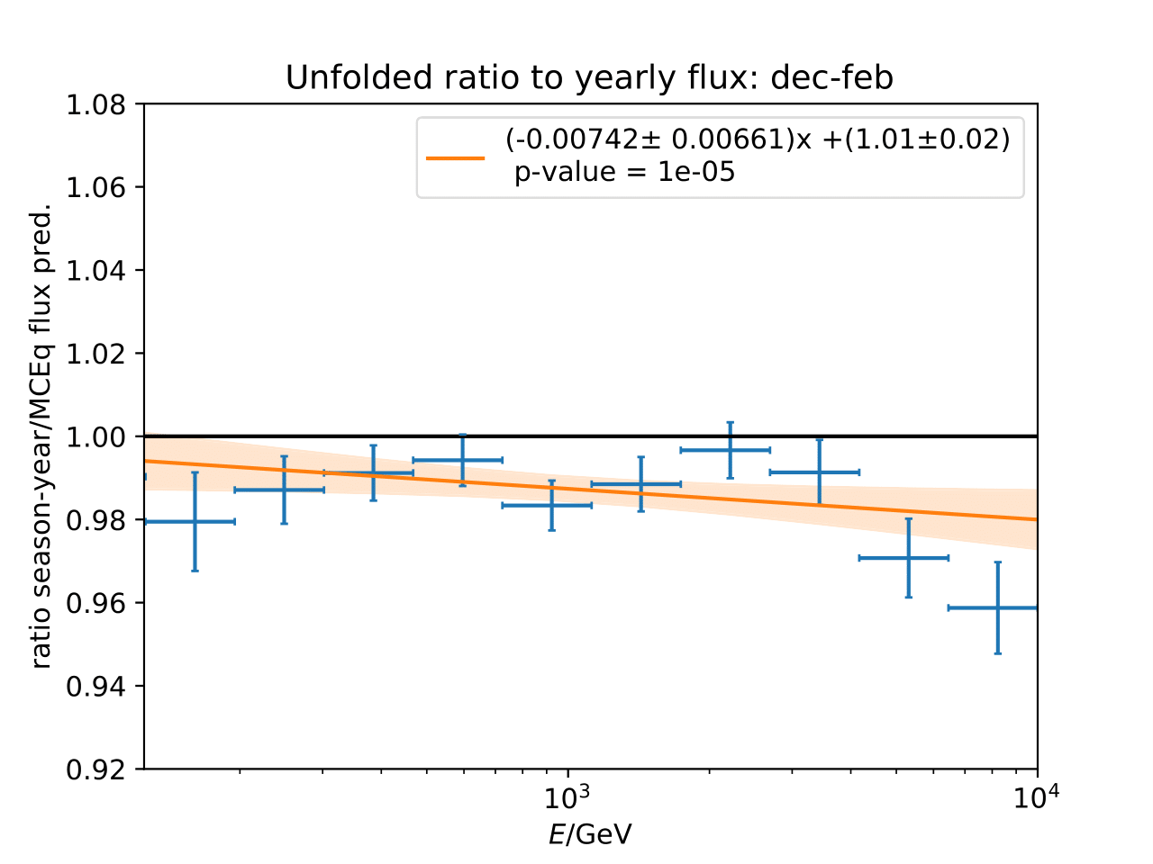
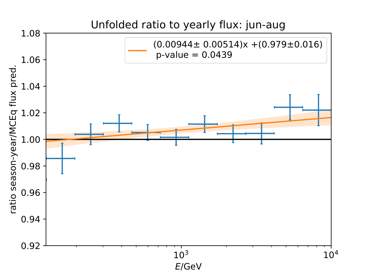
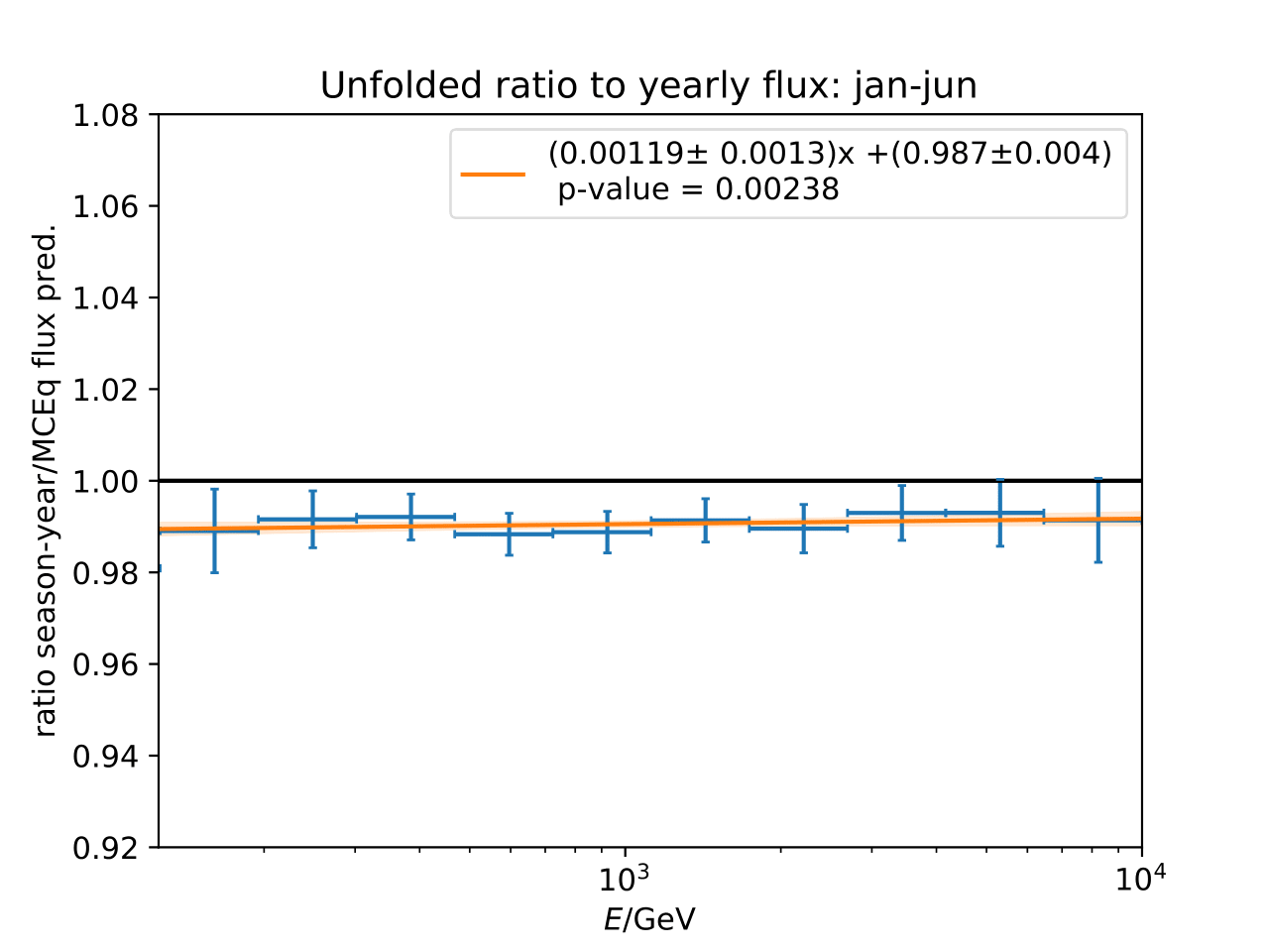
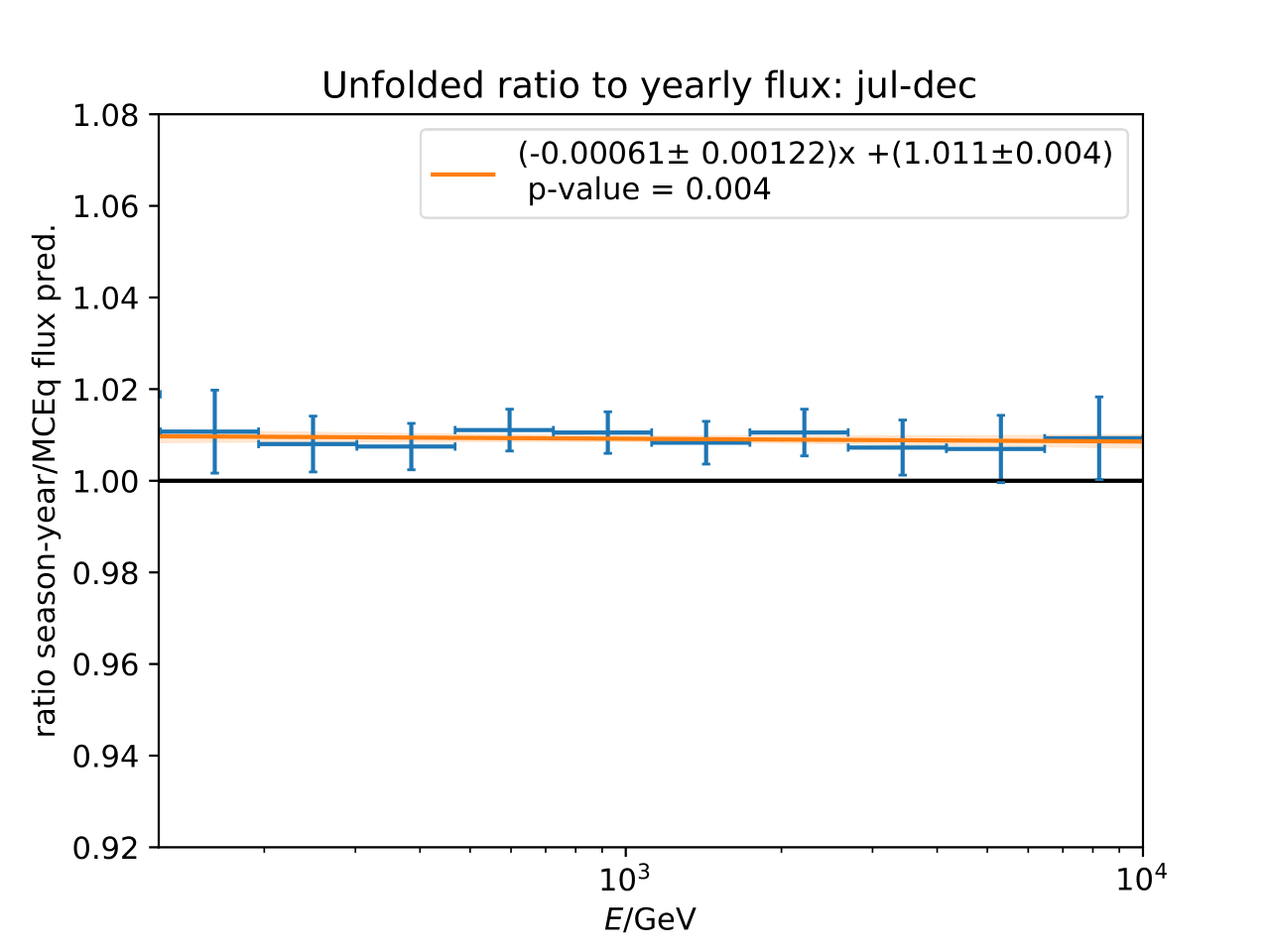
The unfolded ratios are tested against compatibility with MCEq predictions in a \(\chi^2\)-test. Null hypothesis to be rejected is the ratio of 1 (seasonal ratio = ratio from MCEq) Corresponding p-values are listed in the subsequent table. The hypothesis is rejected at a \(3\sigma\)-level.

Compatibility with MCEq (MSIS atmosphere, Sibyll2.3c, H3a)¶
Season	p-value
jun-aug	\(4.39\times 10^{-2}\)
dec-feb	\(7.12\times 10^{-6}\)
jan-jun	\(2.38\times 10^{-3}\)
jul-dec	\(4.00\times 10^{-3}\)
may-aug	\(1.47\times 10^{-21}\)
oct-jan	\(1.73\times 10^{-10}\)
jan	\(1.49\times 10^{-1}\)
feb	\(1.75\times 10^{-6}\)
mar	\(1.08\times 10^{-2}\)
apr	\(8.83\times 10^{-1}\)
may	\(8.78\times 10^{-1}\)
jun	\(3.75\times 10^{-1}\)
jul	\(8.77\times 10^{-1}\)
aug	\(2.04\times 10^{-2}\)
sep	\(3.14\times 10^{-6}\)
oct	\(1.41\times 10^{-3}\)
nov	\(4.38\times 10^{-1}\)
dec	\(2.48\times 10^{-1}\)

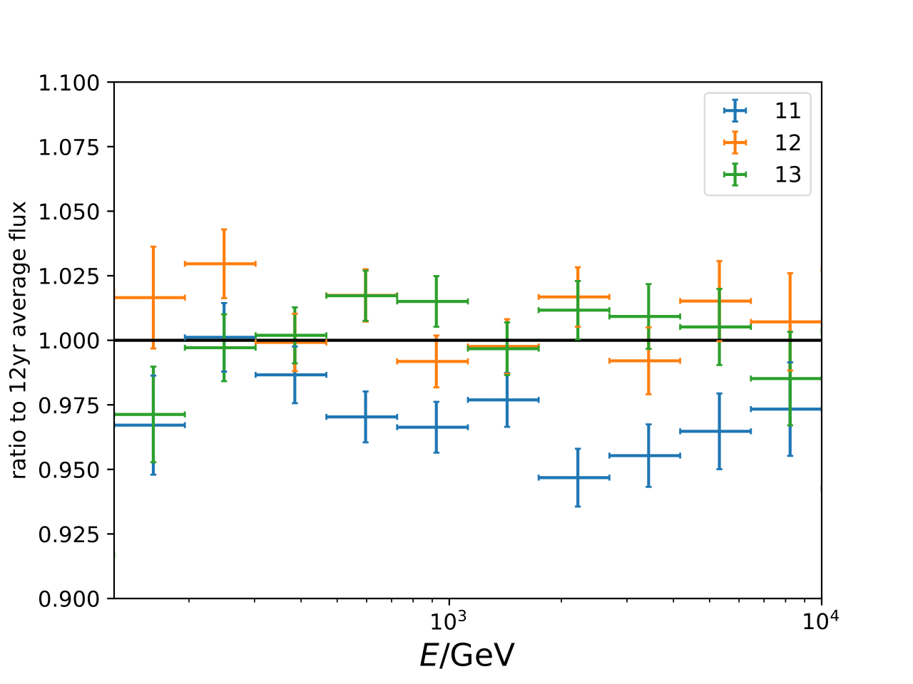
Fit of Variation Strength¶

As presented as post-unblinding plan in the Q&A section, the variations per energy bin and month are determined by a cosine fit: \(A \cdot cos(b \cdot x)\). \(A\) denotes the variation strength in the respective energy bin, \(b\) denotes the period of the cosine. The caps denote the statistical uncertainties of the unfolded ratio of seasonal to annual average flux. Systematic uncertainty averages out, as explained in the wiki. MCEq predictions are shown for comparison.

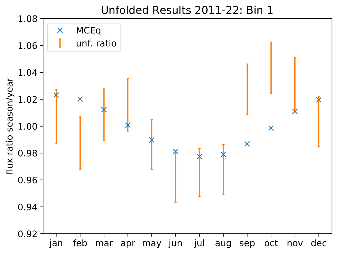
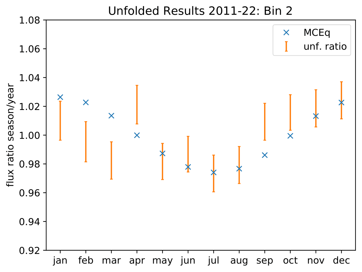
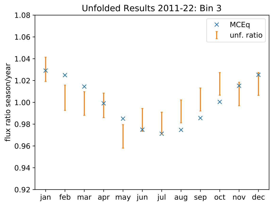
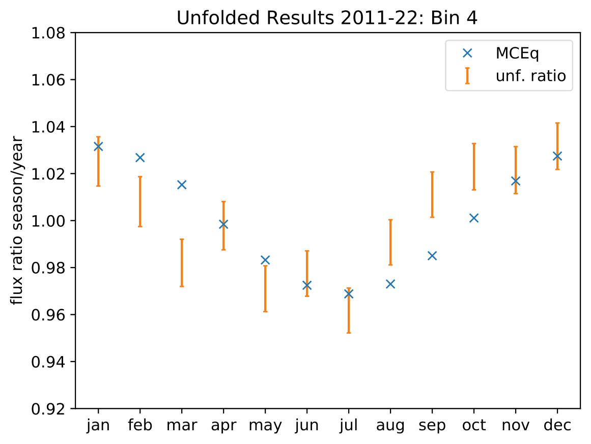
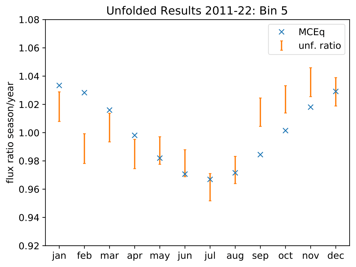
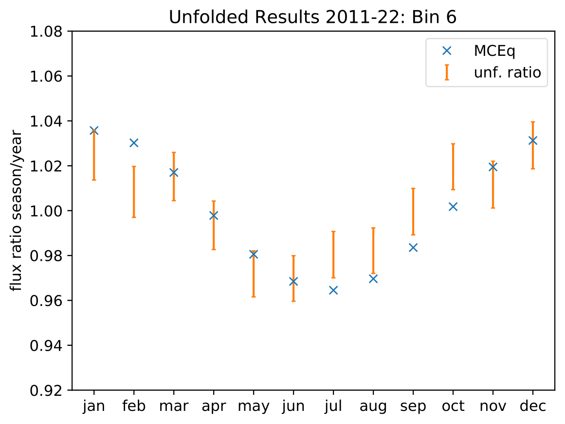
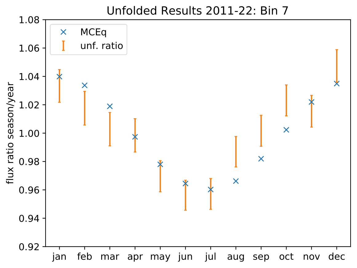
The fit fails for the first 3 energy bins. The discrepancy in fall (August to October) can be observed in the upper plots as well. The period matches the MCEq prediction, however, the variations are shifted. Maximum and minimum deviate in most energy bins.

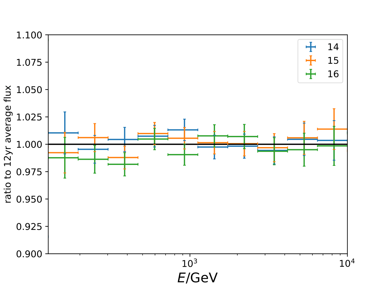
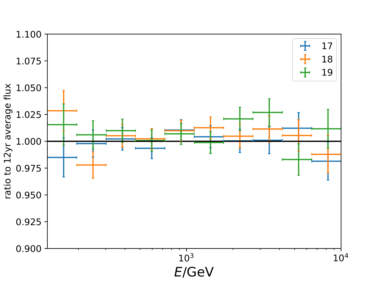
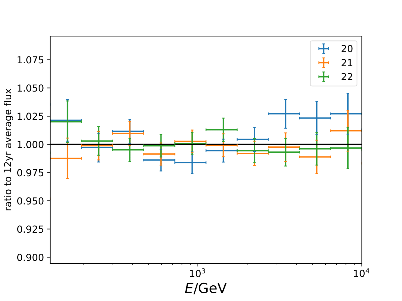
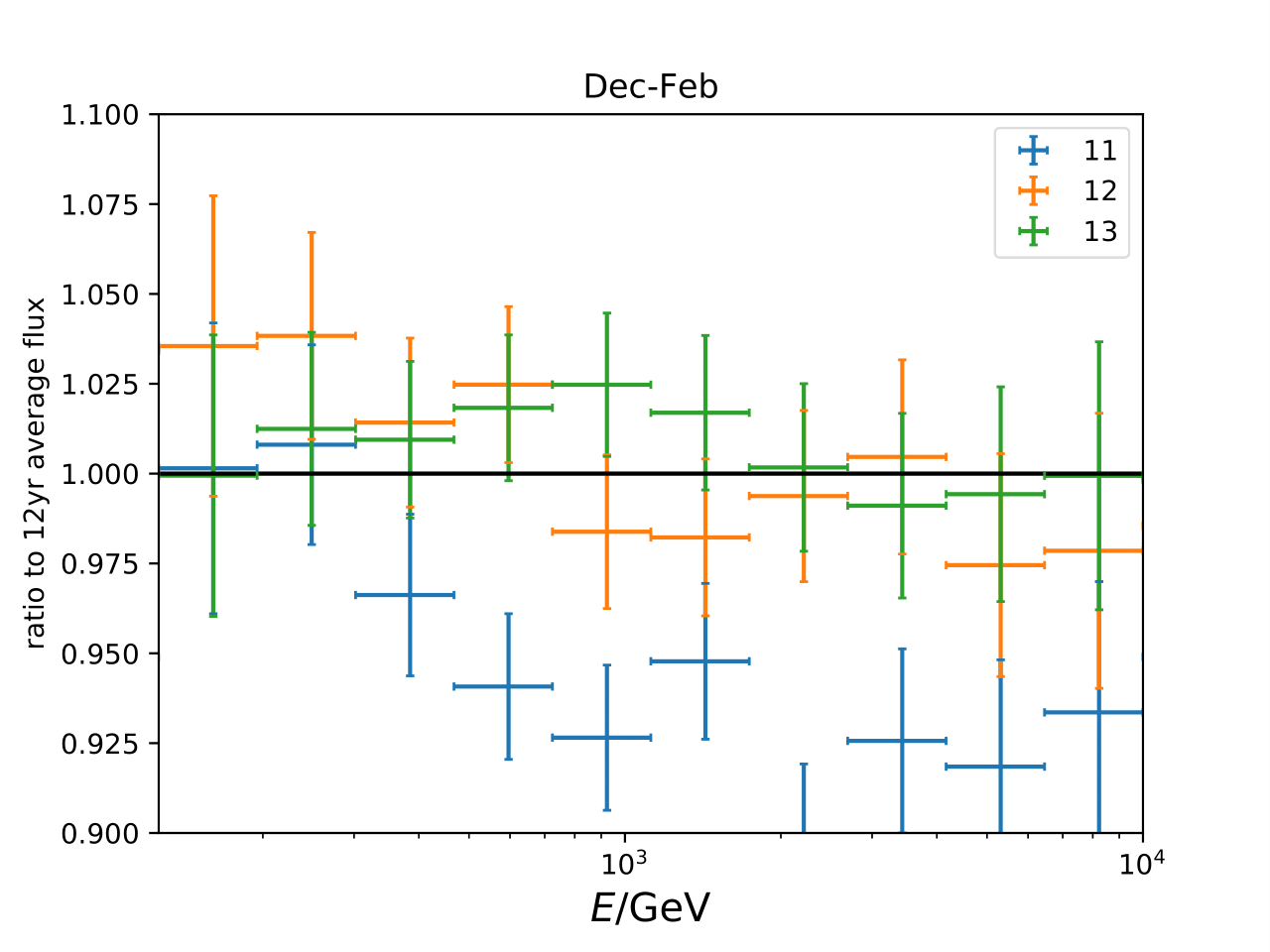
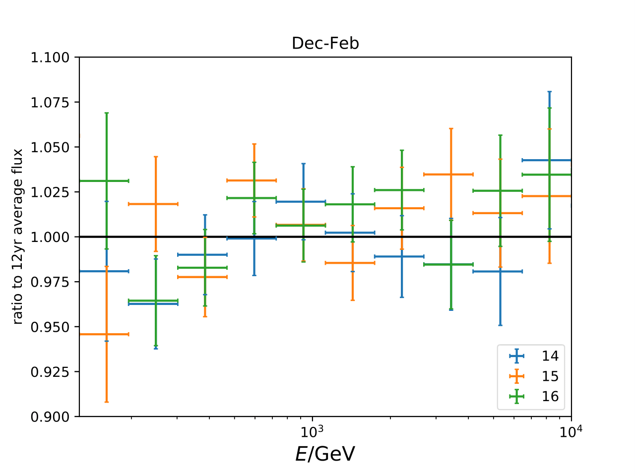
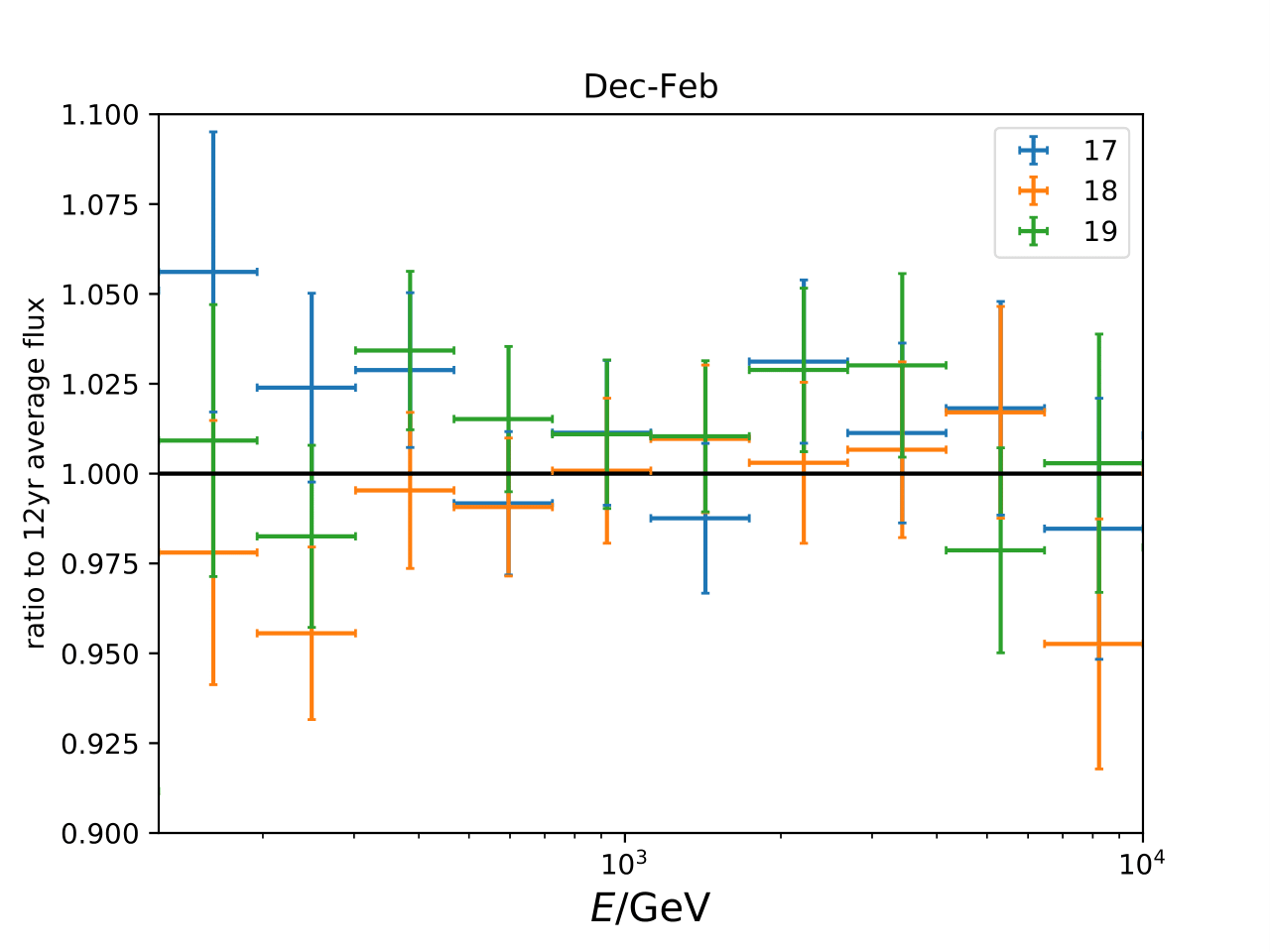
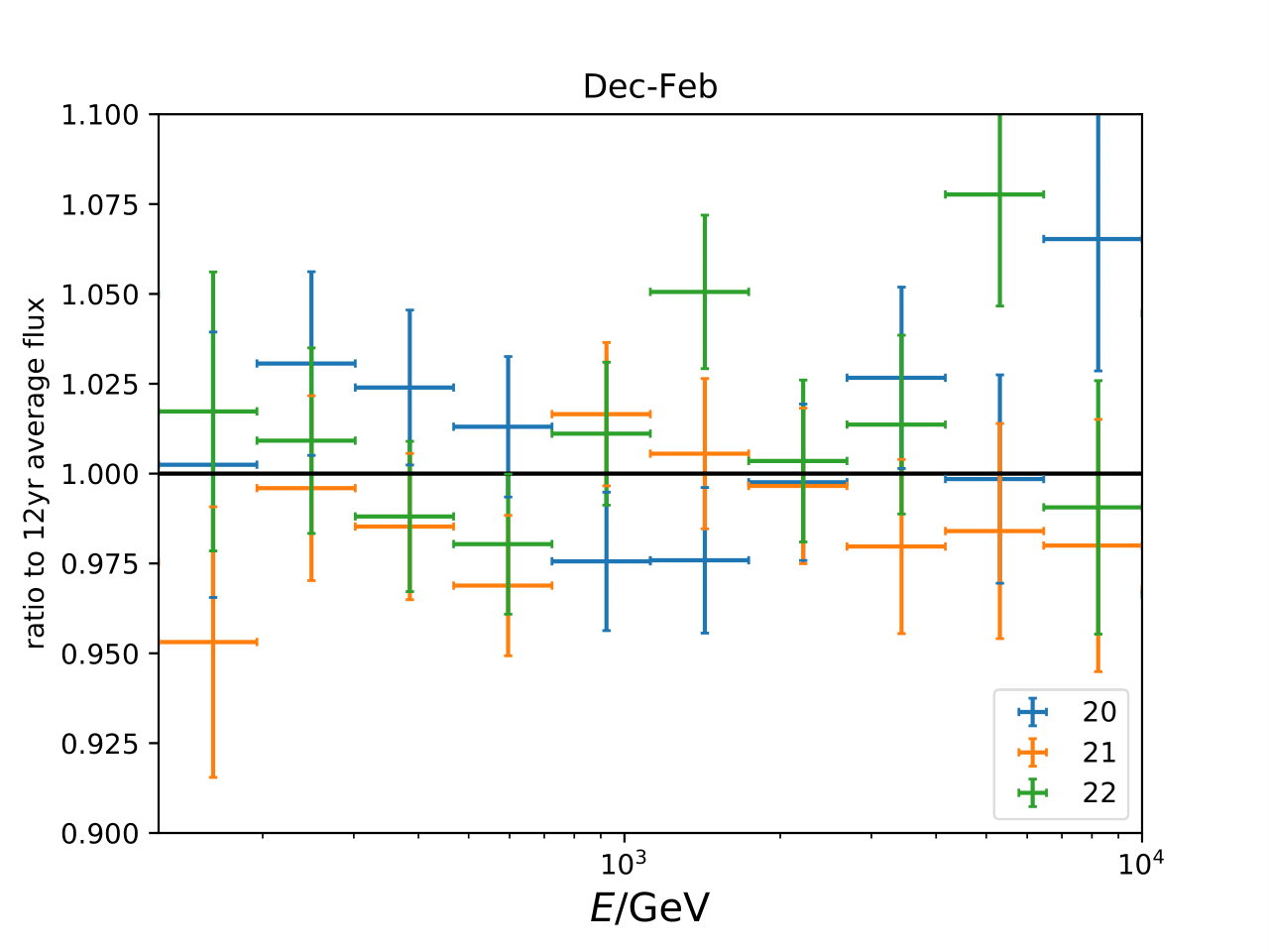
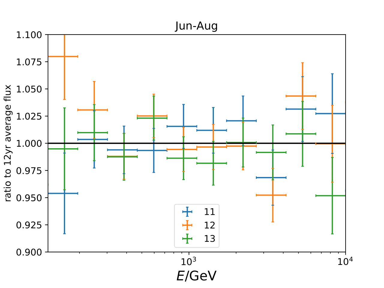
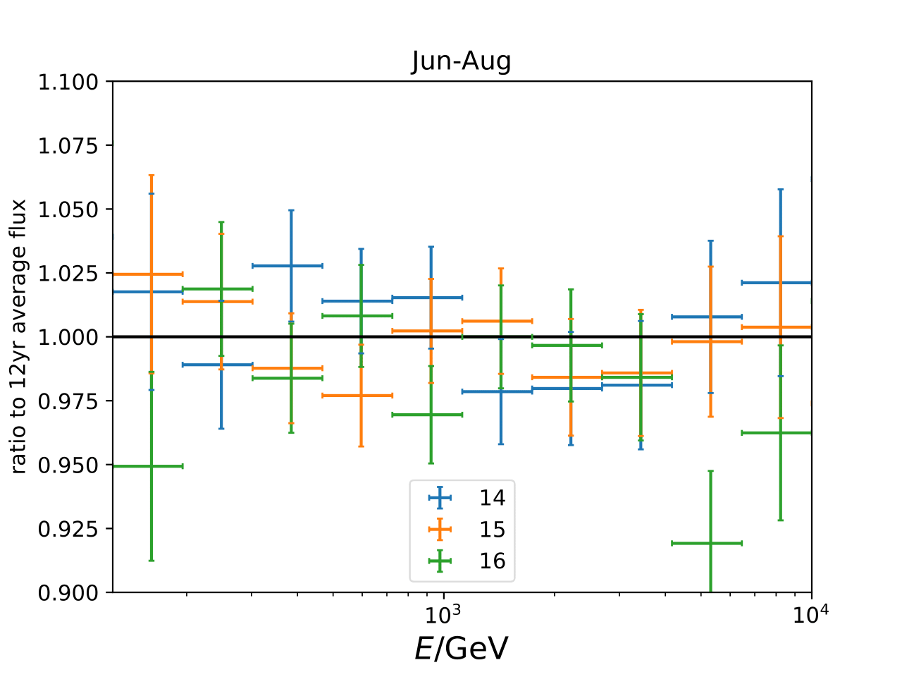
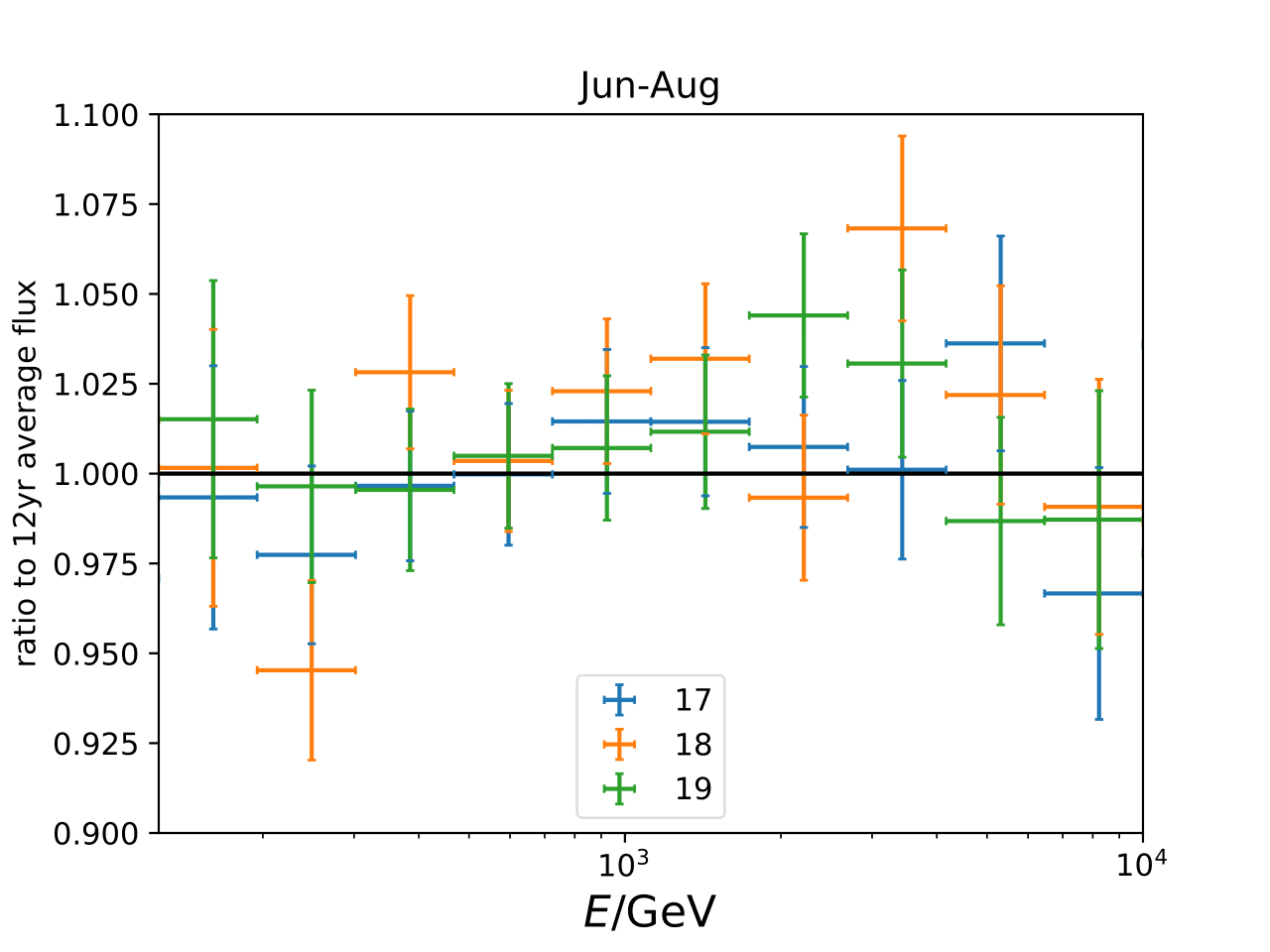
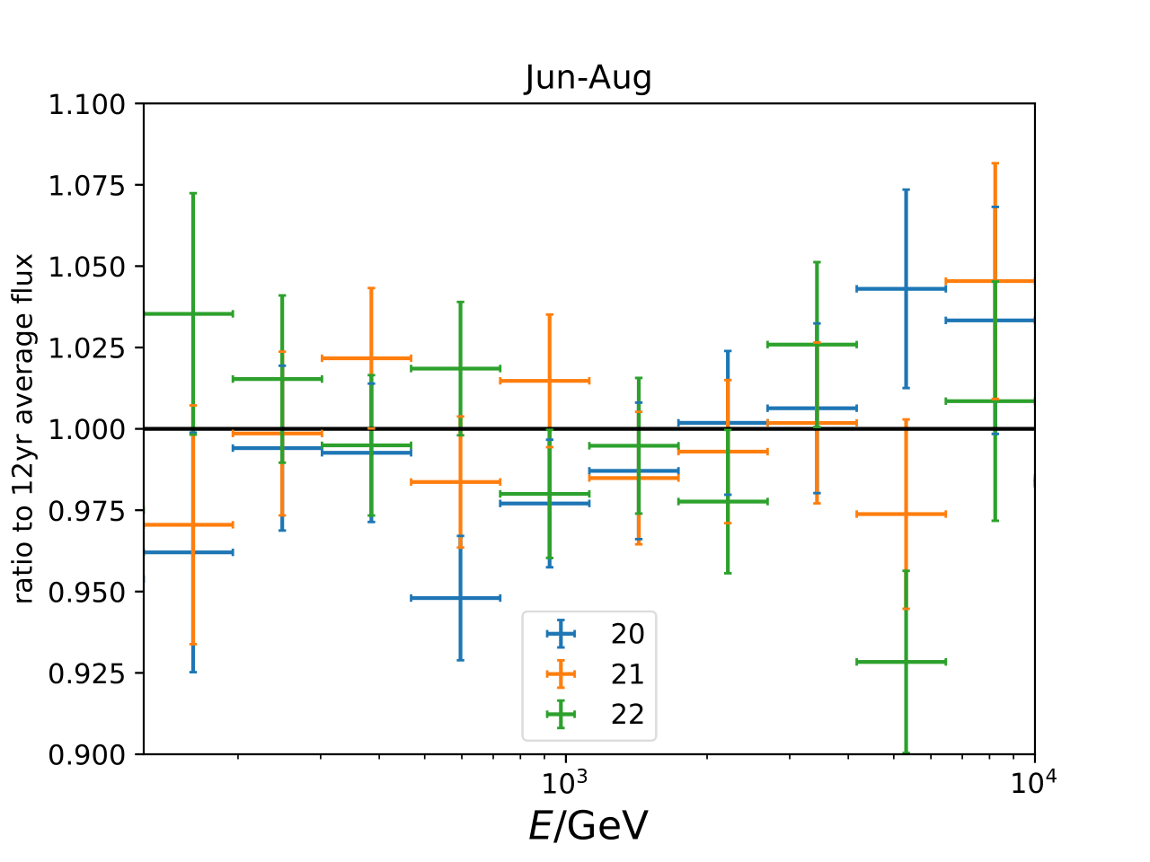
Split into Years - Postunblinding check¶

This section displayed the rejection of data from January 2011 to May 7, 2011 due to old string configuration. The section above contains the curret up-to-date plots after restriction.

These plots were done as crosschecks of the complete 12yrs data set from January 2011 to December 2022. This test revealed that runs from the IC86 string configuration were used.

It is clearly observable that the lower rate of early 2011 causes problems in the unfolded result. Splitting data in combination of three years for summer and winter split (dec-feb vs jun-aug), the dec-feb unfolding yields lower rates than the average 12yr unfolding for the respective season. This behavior is not observable for jun-aug, which is not affected by the changed string configuration.

../_images/yaerlyunfolding_unblind_12yr_2011-13-1.png

../_images/yaerlyunfolding_unblind_12yr_2014-16-1.png

../_images/yaerlyunfolding_unblind_12yr_2017-19-1.png

../_images/yaerlyunfolding_unblind_12yr_2020-22-1.png

../_images/yaerlyunfolding_unblind_12yr_2011-13_dec-feb-1.png

../_images/yaerlyunfolding_unblind_12yr_2014-16_dec-feb-1.png

../_images/yaerlyunfolding_unblind_12yr_2017-19_dec-feb-1.png

../_images/yaerlyunfolding_unblind_12yr_2020-22_dec-feb-1.png

../_images/yaerlyunfolding_unblind_12yr_2011-13_jun.aug-1.png

../_images/yaerlyunfolding_unblind_12yr_2014-16_jun.aug-1.png

../_images/yaerlyunfolding_unblind_12yr_2017-19_jun.aug-1.png

../_images/yaerlyunfolding_unblind_12yr_2020-22_jun.aug-1.png

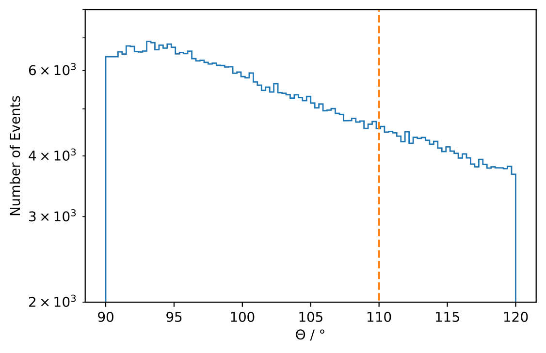
Data-MC Agreement¶

The same data-MC is observable as for the burn sample.

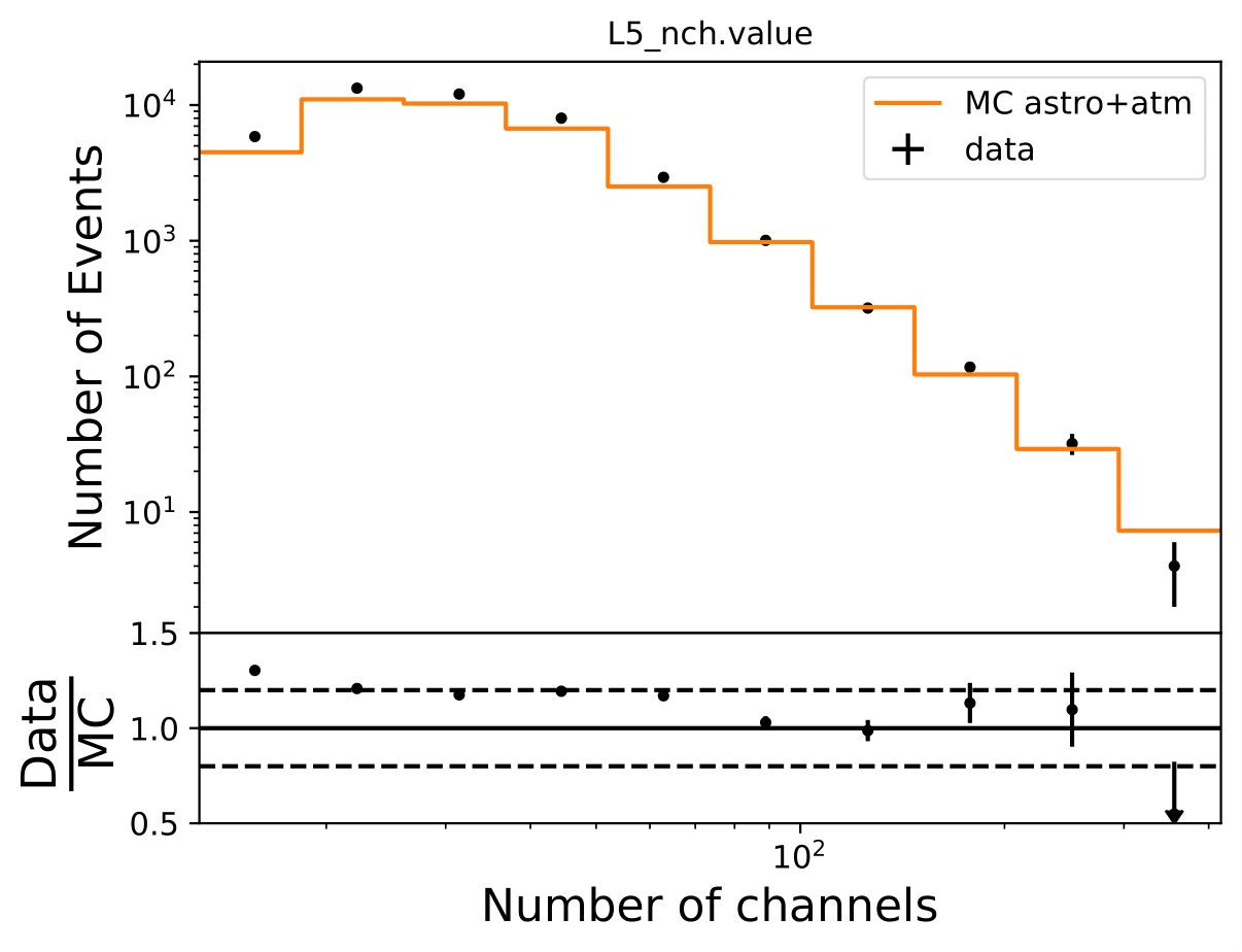
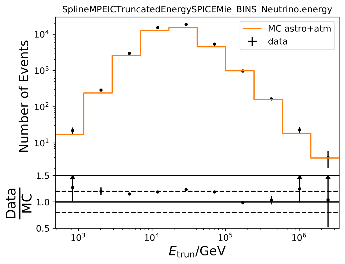
../_images/datavsmc_atmastro_unnormed_L5_nch.value_12yr_21002-1.png

../_images/datavsmc_atmastro_unnormed_SplineMPEICTruncatedEnergySPICEMie_BINS_Neutrino.energy_12yr_21002-1.png

Zenith distribution: