Overview
Atmospheric muon flux
When a cosmic particle hits our Earth’s atmosphere, secondary particles are produced in cascades. Depending on the energy of the primary particle, these cascades are large and produce not only one but several particles. These cascades are called extensive air showers. Since most of the produced particles are unstable, on Earth’s surface mainly neutrinos and muons are detected. The amount of muons arising per area per time interval per solid angle and per energy is called muon flux. This muon flux is divided into two different components, depending on their spectral index \(\gamma\), defined by
One is the conventional component with a spectral index \(\gamma = 3.7\). This flux contains muons arising from pions and kaons, which are the particles produced the most, because they are the lightest hadrons. The other part is build by the prompt component, which are in general all other muons that originate not from pions and kaons. The flux has a spectral index \(\gamma = 2.7\). Thus, it is shifted to higher energies in comparison to the conventional flux. In other words, the prompt spectrum is flatter than the conventional one. The prompt produced particles have short lifetimes which lead in first order to an immediate decay. Hence, the muon energy correlates stronger to the primary particle energy. Instead, the conventional pions and kaons live long enough to interact with the atmosphere. These re-interactions in the atmosphere cause energy losses which reduces the energy successively. This leads to the resulting muons having lower energy as well. Conventional muons dominate below \(1\,\mathrm{PeV}\) and prompt muons dominate above. Figure Fig. 12 shows the different components of the atmospheric muon flux created with MCEq. More information to the hadronic interaction model SIBYLL used to create these spectra are provided here.
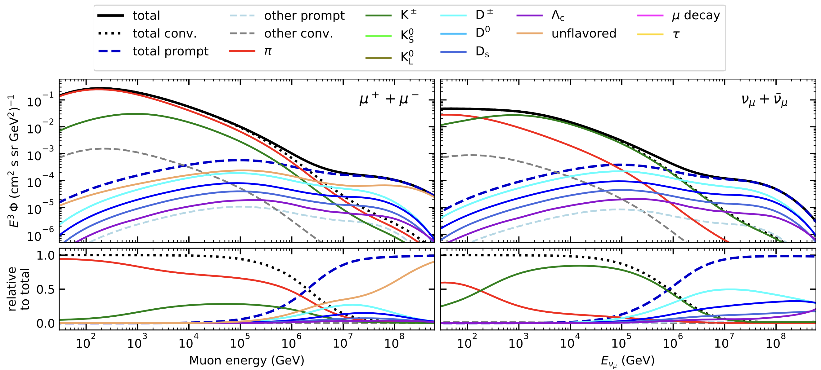
Fig. 12 : The atmospheric muon and muon neutrino flux calculated with MCEq is shown.
Previous analyses
Due to the fact, the resulting muon flux follows a power law, the low statistics at high energies are a challenge to detect the prompt component. In the past, three analyses were performed focused on high energetic muons arising from our Earth’s atmosphere by Thomasz Fuchs, Patrick Berghaus and Hans-Peter Bretz. In Tomasz’s thesis, which included an unfolding of the energy spectrum with one year of experimental data, the analysis was limited by MC statistics. This caused the analysis to result in a prompt normalization that is compatible with zero. In Patrick’s thesis, a mismatch between MC and data was found in the \(\cos(\theta)\) distribution, which could not be resolved. The detection of the prompt component was done with \(3.5 \sigma\), for the primary flux model of Gaisser H3a, for example. The largest uncertainty arises from the assumption of the primary flux model. Hans-Peter performed an analysis with three years of data, but a final muon spectrum as a function of the actual muon energy has never been derived.
The links to the analyses can be found here.
New analysis
Our new analysis focuses on two main goals. The central part of this work is the unfolding of the atmospheric muon energy spectrum, which allows us to measure the flux and identify the contribution from the prompt component. The second goal is to develop a method to perform a forward folding fit of the prompt contribution, which can be used in future analyses.
In earlier analyses, the distinction between prompt and conventional muons could not be made directly, since the parent particle information was not stored in the CORSIKA simulations used in IceCube. To classify a muon as prompt, the type of its parent particle needs to be known (see prompt definition). However, this information was previously omitted because it requires additional disk space and is not essential for neutrino source searches.
By enabling the EXTENDED HISTORY option in CORSIKA, the parent and grandparent particles of each muon can now be stored in the I3MCTree. We have started producing such simulations, which makes it possible to separate the atmospheric muon spectrum into prompt and conventional contributions. In principle, this allows us to apply a scaling factor to adjust the relative fraction of prompt and conventional particles. The value of this scaling factor corresponds to the prompt normalization that can be obtained in a forward folding fit.
Since the production of sufficiently large CORSIKA samples at high energies requires several months of computing time, this scaling method enables a forward folding approach without the need to rerun large-scale simulations for different hadronic interaction models. This saves resources and avoids the complexity of retuning interaction models, which typically requires close collaboration with the model builders.
While the current analysis presented here is focused on the unfolding of the muon spectrum, we are also developing a forward folding approach using this scaling method, which will be presented in the near future. Stay tuned!
Analysis Overview
The Figure below represents an overview of the entire analysis chain. At first, new simulations have been generated using CORSIKA. Then, all reconstructions are machine learning based, utilizing convolutional neural networks (CNNs). The event selection is done in 4 steps. At first, the muon filter is applied to select muons. Then, an energy cut is performed to remove low-energetic muons. To select well-reconstructed and contained events, data-MC quality cuts are performed. At last, a cut on the leadingness is applied to select events where the leading muon carries most of the energy of the muon bundle. This sample is then used to unfold the atmospheric muon flux.
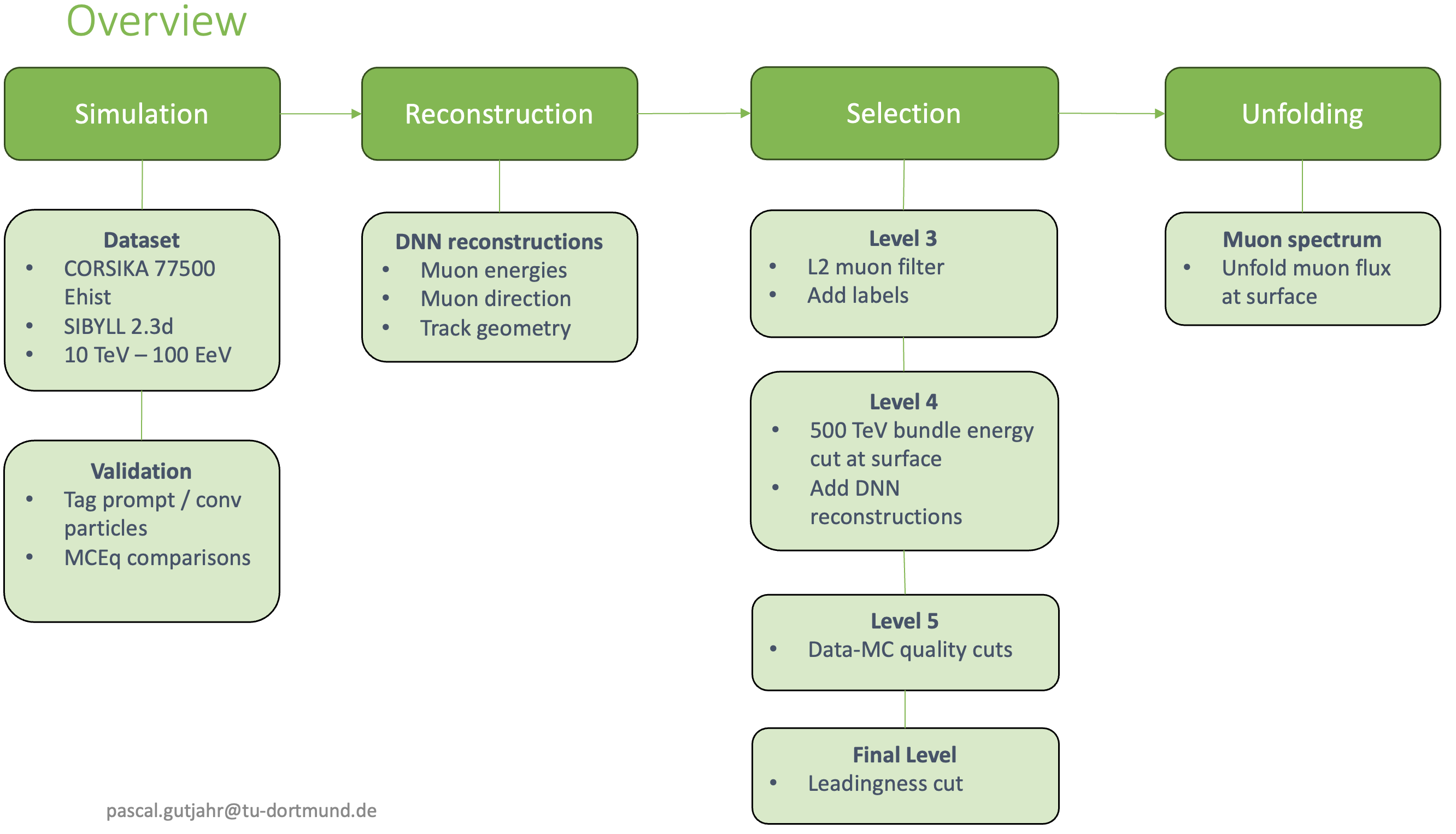
Fig. 13 : Overview of the entire analysis chain.