Q & A
In this section, a collection of all questions and answers from the presentations is given. The presentations are listed here.
October/November 2025, (Collab review)
Q (Anatoli): What is the impact of the regularization strength on your unfolding results?
A: The regularization strength is determined by minimizing the bin-to-bin correlation of the unfolding bins. For this, a polynomial of fourth order is fitted to the global correlation. I created a test to estimate the impact of the regularization strength. In addition to the minimum of the fitted polynomial, I also calculate a lower and upper \(\tau\) value, where the global correlation is increased by \(0.5 \%\). In the example shown in Fig. 242, this results in a deviation larger than 20 % in the regularization strength.
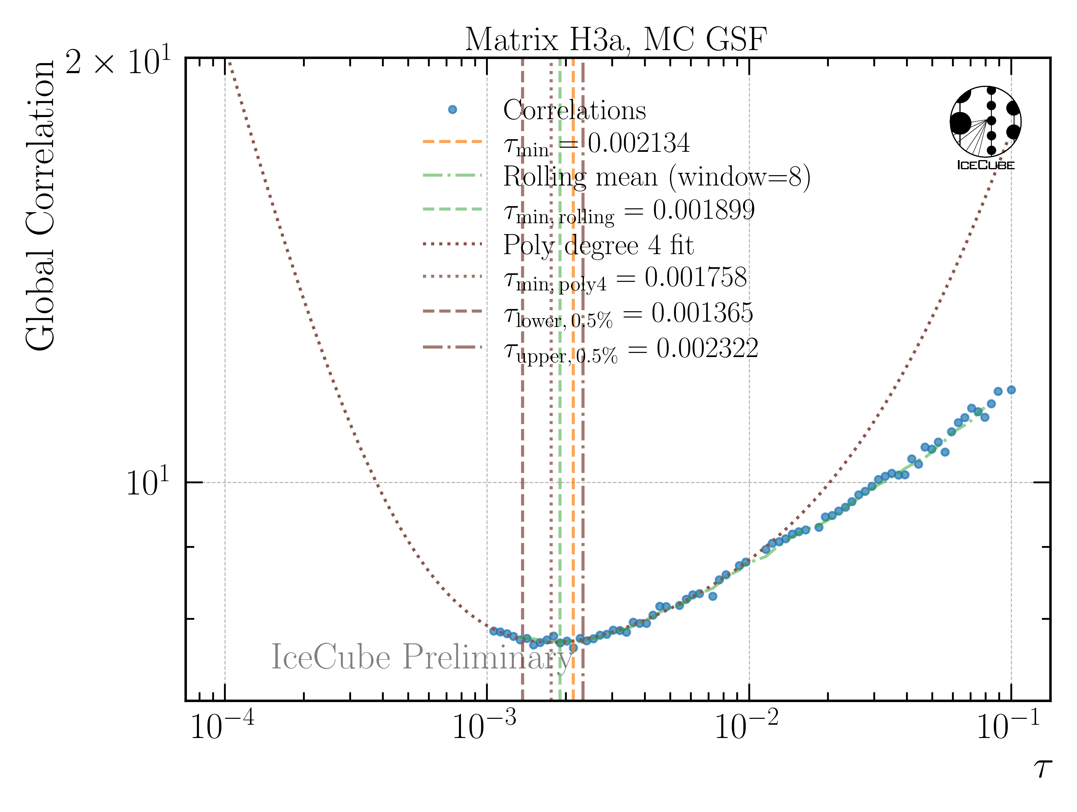
Fig. 242 : Global correlation as a function of the regularization parameter tau.
When I unfold with the lower, upper and best fit tau value, I obtain the results shown in Fig. 243.
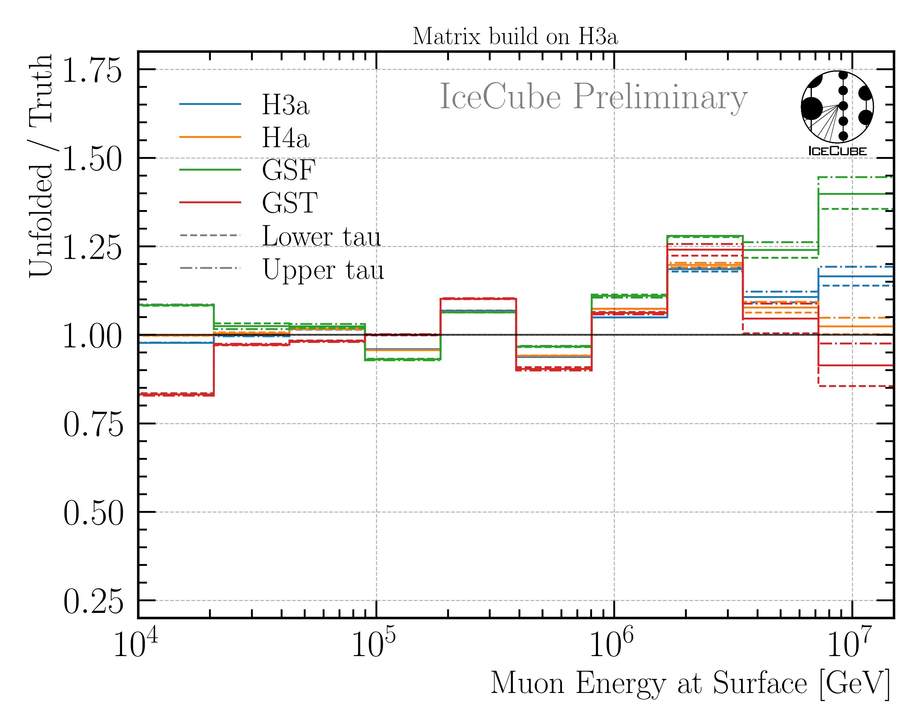
Fig. 243 : Impact of the variation of the regularization strength on the unfolding.
To estimate the impact of the regularization strength only, I then divide the unfolding results with the lower and upper tau by the unfolding with the best fit tau. This is shown in Fig. 244. The impact is below 10 %. This impact is smaller than the statistical uncertainty per bin in Fig. 10, thus, this uncertainty is not included as an additional systematic uncertainty.
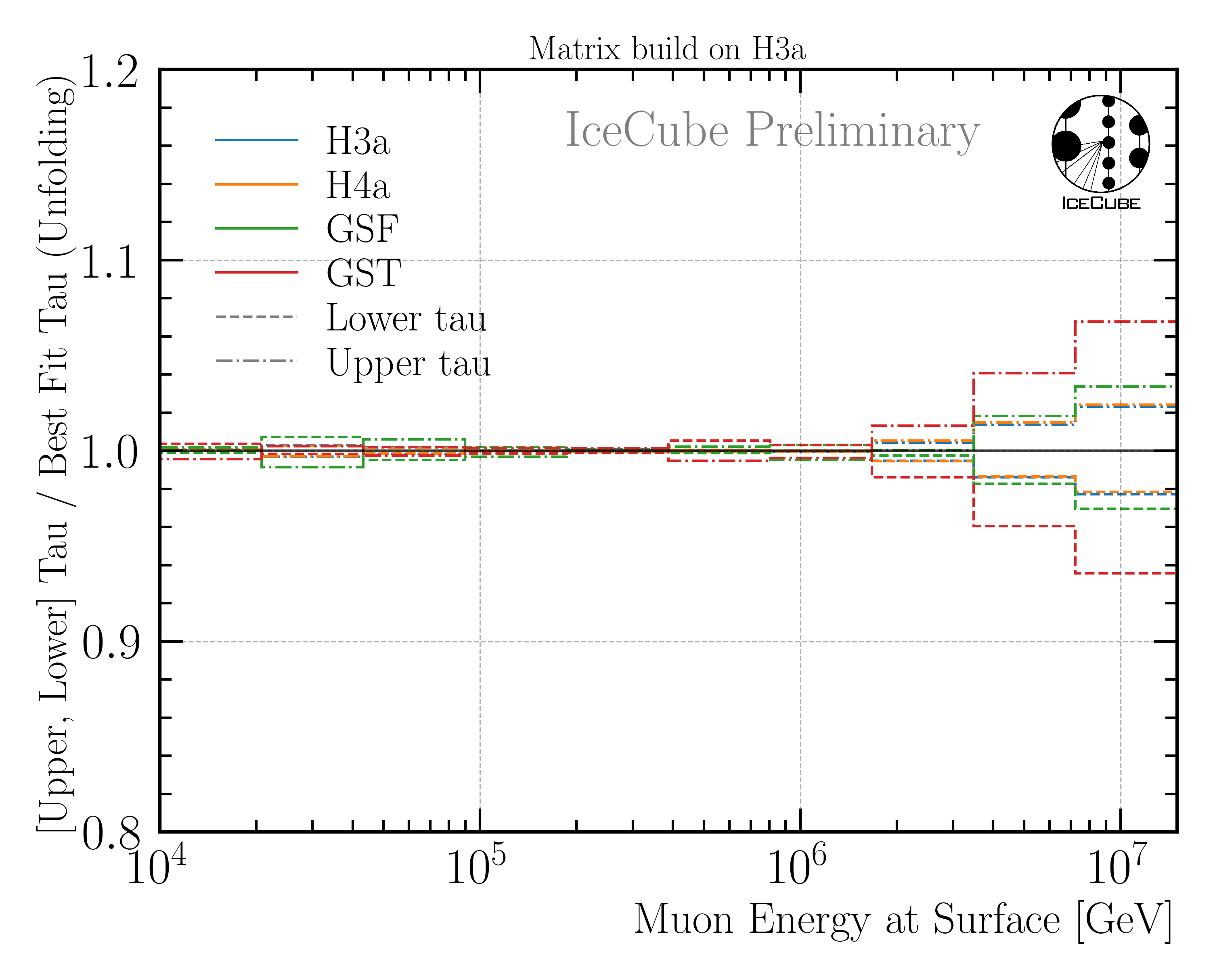
Fig. 244 : Unfolded muon flux for lower and uppwer tau, divided by the unfolding with the best fit tau. This shows the impact of the regularization strength on the unfolding result.
Q (Anatoli): Can’t you treat the regularizatipon strength as a free parameter in the unfolding?
A: Treating the regularization strength as a free parameter in the unfolding is not possible. The Regularization term is added to the likelihood, thus, for the minimization of the likelihood the optimal regularization strength would always be infinity because it scales by \(1/\tau\).
Q (Anatoli): It looks like the unfolding has a bias. Depending on the unfolding bin, there is a deviation between the true MC distribution and the unfolded MC distribution. How do you treat this bias?
A: This is correct. The deviation is treated as a systematic uncertainty, and it is added in quadrature to the total uncertainty. The bias is presented in Fig. 8.
Q (Anatoli): How do you determine the prompt component from your unfolded flux?
A: A \(\chi^2\) fit is performed. This is done for several assumptions (different primary models). The fit includes a normalization factor for the prompt and conventional component. More details are provided in Flux Characterization.
Q (Anatoli): Could you show the uncertainty contribution on each bin from the different systematics/sources?
A: Yes, this is presented in Fig. 10.
September 17, 2025
Q (Anatoli): What is the impact of the hadronic interaction model on your unfolding?
A: This is an important question, however, it is technically not possible to perform the unfolding with different hadronic interaction models, since we would need to simulate several datasets with different hadronic interaction models. The current simulation I am using is based on SIBYLL 2.3d, and I have started the simulation 1,5 years ago, and it is still running. Thus, producing several CORSIKA sets is not feasible. Instead, we can estimate the impact of the hadronic interaction model based on MCEq. In Fig. 245, the flux of muons at the surface is shown for different hadronic interaction models. The fluxes are calculated using MCEq assuming the GSF primary model. The ratio panel presents the total fluxes in relation to SIBYLL 2.3d. If we now look at Fig. 246, the flux of muons at the surface is shown for different primary models. The fluxes are calculated using MCEq assuming SIBYLL 2.3d as hadronic interaction model. The differences between the different hadronic interaction models are smaller than the differences between the different primary models. Hence, we can estimate that the impact of the hadronic interaction model on our unfolding is smaller than the impact of the primary model, and for the primary model we have shown that there is no significant impact on the unfolding, as presented in Fig. 236.
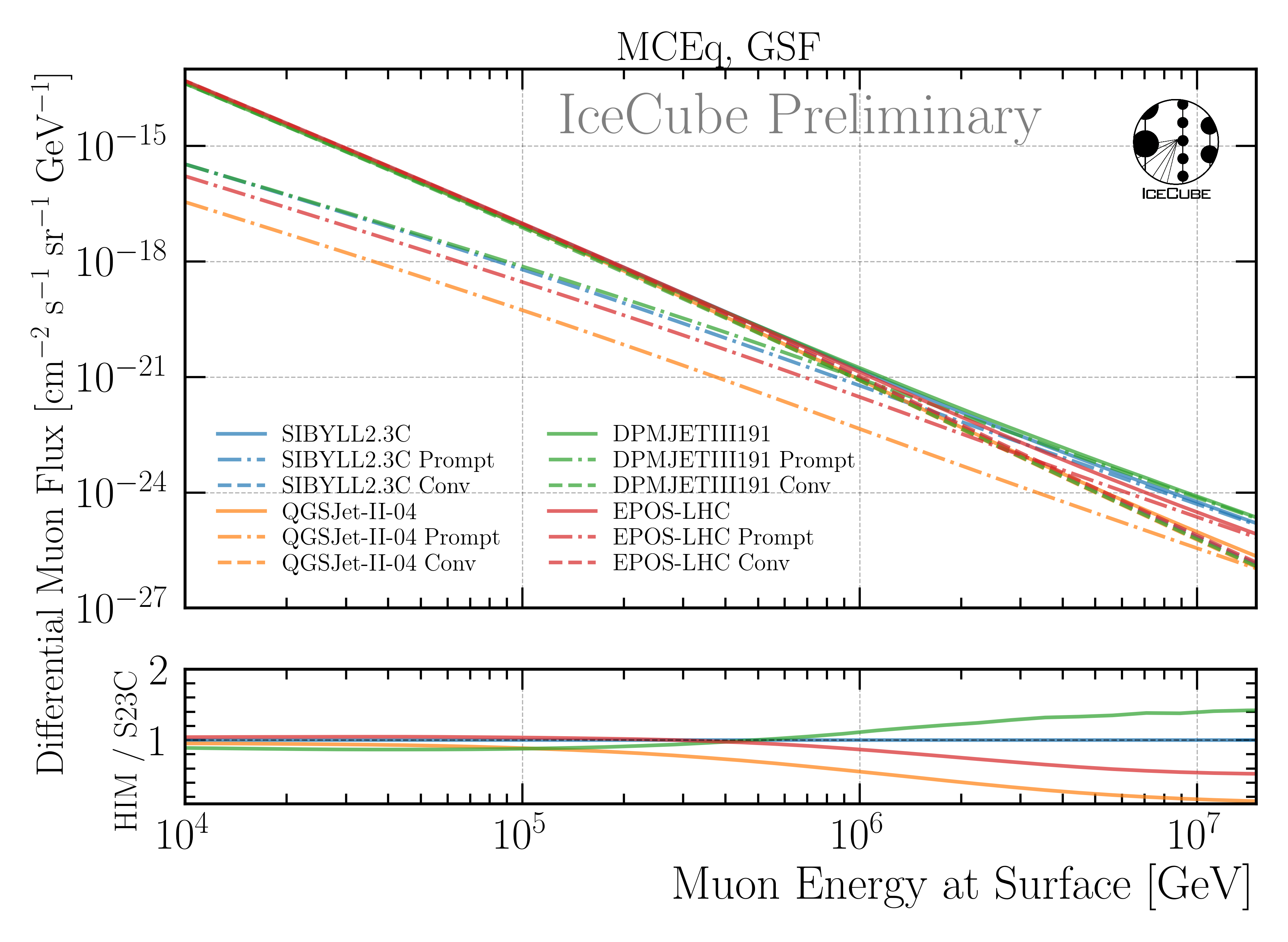
Fig. 245 : The flux of muons at the surface is shown for different hadronic interaction models. The fluxes are calculated using MCEq assuming the GSF primary model. The ratio panel presents the total fluxes in relation to SIBYLL 2.3d.
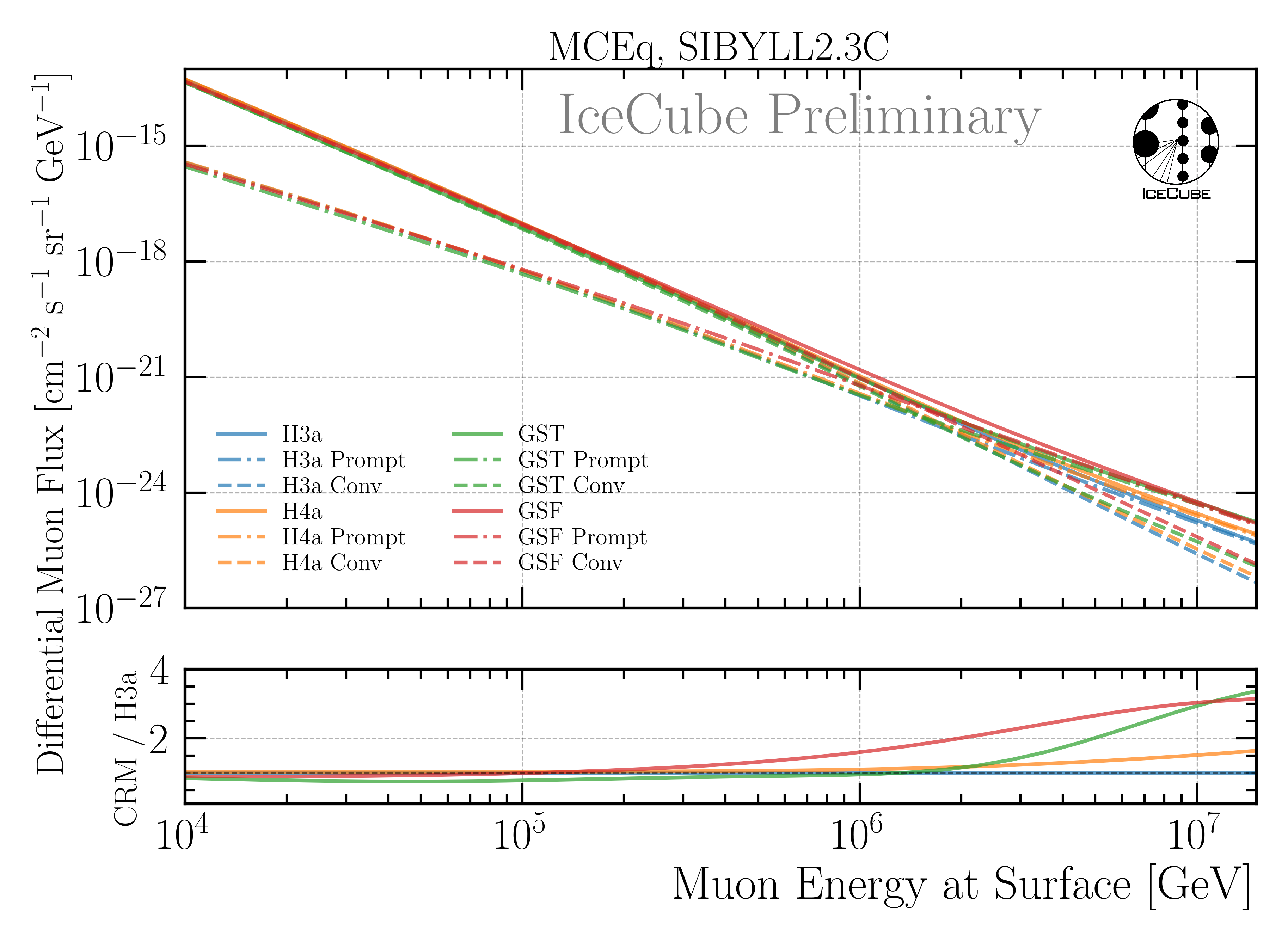
Fig. 246 : The flux of muons at the surface is shown for different primary models. The fluxes are calculated using MCEq assuming SIBYLL 2.3d as hadronic interaction model. The ratio panel presents the total fluxes in relation to H3a.
August 15, 2025
Q (Dennis): Does a background event impact the reconstruction of the leading muon energy at entry?
A: On slide 10, I have presented the reconstruction for events without a background event, for events with a leadingness below 0.1, and for a leadingness above 0.1. Given the statistics, there is no significant impact on the reconstruction. Since the networks are trained on events with background primaries, the networks have already seen these event signatures.
Q (Stef): How do you propose to treat the systematics?
A: The LLH minimization in the unfolding using minuit provides the full covariance matrix. This includes, the under and overflow bin, the actual unfolding bins, and the 5 ice systematics. I run the unfolding once. Then I take the best fit values of all 5 ice systematics and scale them them up and down by it’s fitted uncertainty, coming from the covariance matrix. I then run the unfolding again with these fixed ice systematics. Scaling 5 systematics up and down results in 10 unfoldings in total. For example, the best fit of absorption is 1.01±0.01, then I fix it to 1.02 and 1.00. In this example, all other four systematics are fixed to their best fit value. Then I calculate a systematic uncertainty via
with \(i\) being the 10 unfoldings, \(f_{\mathrm{baseline}}\) the initial unfolding, and \(f_i\) the unfolding with one systematic scaled up or down. The total uncertainty is then calculated via
with \(j\) referring to the different systematics (absorption, scattering, etc.) thus \(M\) is 5. The statistical uncertainty is then estimated via the poisson distribution assuming \(\sqrt{N}\) uncertainty in each bin. I propose this uncertainty estimation, however, Anatoli has not fully agreed on this yet. Thus, for now, I stick with the systematic uncertainty estimation resulting from the effecetive area variations, as presented in Unfolding/Effective Area. This estimation is more conservative since not fitted information are included in the effective area variations. A tighter uncertainty estimation utilizing the fitted ice parameter makes sense, and can also be included after the unblinding.
Q (Dennis): The background event rate is quite high. It looks like your selection prefers events with background primaries. Do you know why and did you check the rates for your background distribution?
A: For my selection, with a leading muon energy at surface above 10 TeV, the background rate is 0.58 mHz, and the signal rate is 0.74 mHz. With a requirement that the coincident muon bundle at surface contributes at least to 10 % to the signal energy at surface, the background rate drops to 0.02 mHz. This 10 % estimate is chosen approximately, since the reconstruction of the leading muon energy would not be significantly impacted by a coincident muon bundle with a lower energy. I can’t say, why the selection prefers events including a background primary. This was presented in Systematics Update and Coincident Primaries.
Figure Fig. 247 shows the contribution of coincident events to the muon events at surface. The asymmetry \(a\) is defined as
with \(E_{\text{leading}}\) being the leading muon energy at surface, and \(E_{\text{bundle,coinc}}\) being the energy of the coincident muon bundle at surface. Thus, a value of 1 means that there is no coincident muon bundle, and a value of -1 means that the coincident muon bundle dominates over the target leading muon. The asymmetry is shown as a function of the leading muon energy at surface, the target unfolding variable. The plot shows that for leading muon energies above 10 TeV, there are almost no coincident bundles with higher energies than the target leading muon. For a few outlier events, the coincident bundle contributes 25-50% to the total energy at surface. However, for most of the events, the coincident bundle contributes only a little, considering the yellow row at the top of the plot, based on the logarithmic color scale. This is expected, since we have a powerlaw distribution and thus the higher the energy, the less often do these events occur, and thus the probability of having two high energetic primaries in one event is low. Since 10 TeV is the lower bound of the unfolding, the impact of coincident bundles is low/negligible.
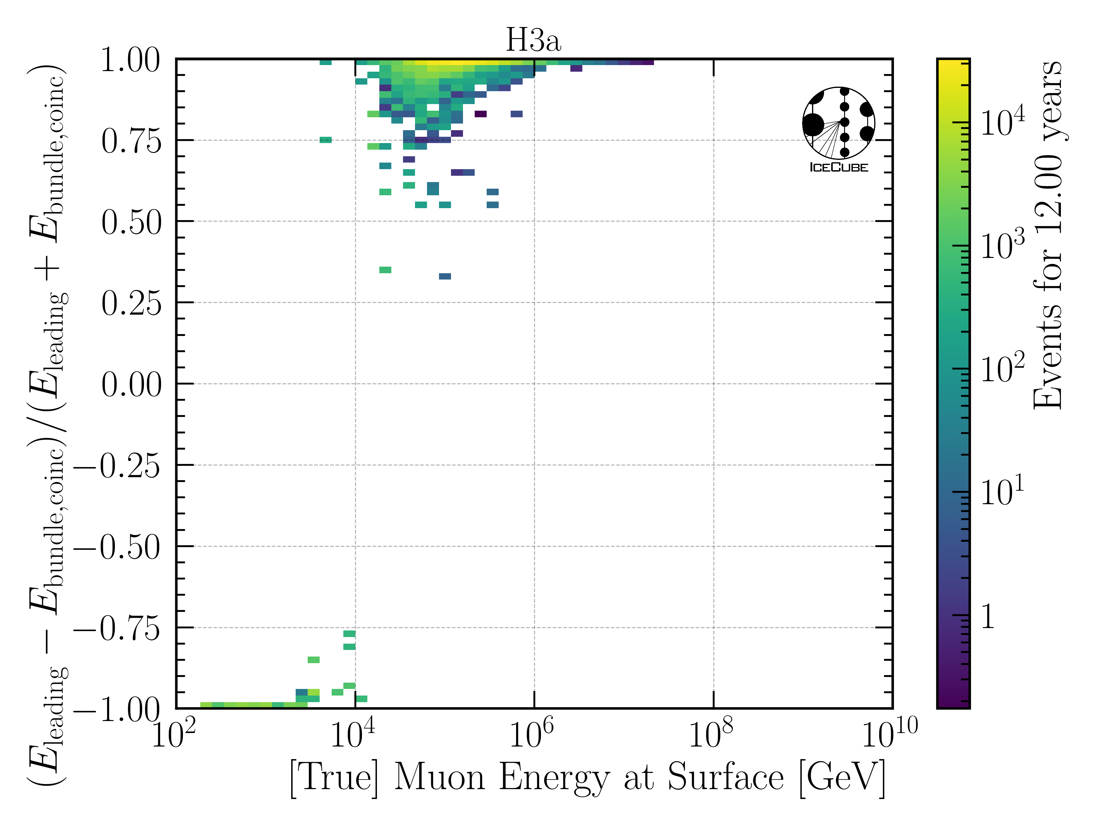
Fig. 247 : Contribution of coincident muon bundles to the target leading muon at surface. Below 10 TeV, the energy of the coincident bundle is higher than the target leading muon energy for most events. Above 10 TeV, the coincident bundle contributes only a little to the total energy at surface. Since 10 TeV is the lower bound of the unfolding, the impact of coincident bundles is negligible.
June 27, 2025
Q: How is leadingness reconstruction performed?
A: DNN reconstruction. Leading energy divided by bundle energy at entry.
Q: Sensitivity to different components of prompt?
A: Not with unfolding, it measures an inclusive flux. For forward, tested shape differences but probably not possible at our energies.
Q (Dave): Could leadingness reco be useful for single/bundle separation, specifically for leading muon with faint bundle?
A: Probably, might need training on sample including neutrinos.
April 1, 2025 (CRWG review)
Q (Dennis): I think many aspects described in the “physics motivation“ part should go in the “Overview“ section. For example, you explain air showers here. If you want to keep this explanation, I think it belongs to the Overview. Also, it would not harm to move the goals of this analysis to the Overview section. Otherwise, I think this section is great.
A: I agree that some parts of the physics motivation explain basics like air showers. However, here I just want to give a short introduction to explain the physics relevant for the machine learning based reconstructions. For example, that not only one muon but several muons were created and detected in the in-ice array. The goals are also mentioned in the overview section. I mentioned them in the CNN section again to introduce the section. Thus, I would like to keep the physics motivation as it is.
Q (Dennis): Pascal: “This flux contains muons arising from pions and kaons, which are the particles produced the most in the first interactions, because they are the lightest hadrons.” — Sry, what exactly is incorrect here? Dennis: Well, I guess strictly speaking the statement is not wrong, however, why do you single out the first interaction (this is what I was referring to)? Pions and kaons are the most abundant ones in all interactions (because they are the lightest hadrons). I don’t understand the relevance of the reference to the 1st interaction here.
A: OK. You are right, the “first interaction” is not necessary. I removed it.
Q (Dennis): I think the part “v1.11.0-rc1 code fix“ in “New CORSIKA Ehist IceProd simulation“ could also go into the appendix as it is not needed for the analysis review.
A: The appendix includes all information about our first test simulations, referred to as datasets 30010-30013. I agree that the code fix for the new simulation is not needed for the analysis review, however, this chapter is not very long and I would like to keep it here to make sure there was a minor code fix in case somebody wants to reproduce the simulation.
Q (Dennis): One question that arises from the CORSIKA settings: You do not simulate coincident events, but data will include coincident events. Can you show that this does not cause any problems? Is there any dedicated selection to remove coincident events? If not, which of the cuts removes them?
A: In Fig. 248, the probability of having coincident primary particles is shown. For a time window of 6 µs, the probability of having a coincident primary particle with an energy above 10 TeV is lower than 1 %. The time window of 6 µs is achieved by the time window cleaning applied to the pulses used for the DNN feature generation, as described here. For the probability calculation we assumed that the DNN reconstruction would reconstruct the energy of the muon with the higher energy, in case there are two or more muon bundles entering the detector. Furthermore, for the unfolding, we will have a lower energy limit of muon flux at surface of 10 TeV, which obviously requires a primary energy even higher than 10 TeV and the probability of having coincident primary particles decreases with increasing primary energy.
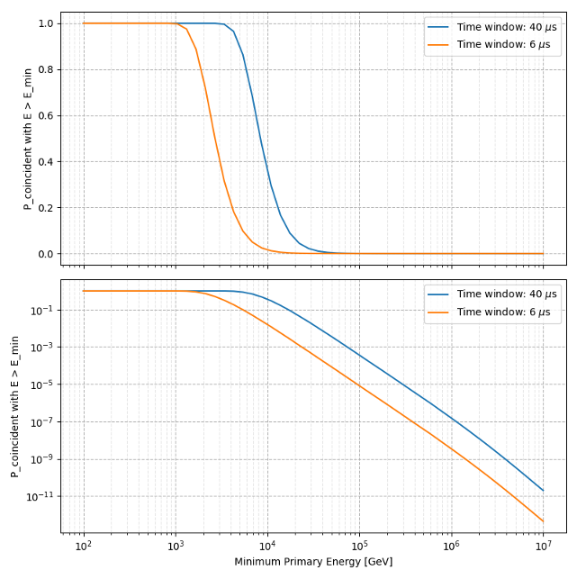
Fig. 248 : The probability of having coincident primary particles is shown. The top panel shows a linear y–scale, the bottom panels shows a logarithmic y–scale. Above 10 TeV, the probability of having a coincident primary particle with an energy above 10 TeV is lower equals 1 % for a time window of 6 µs.
Q (Dennis): Datasets 30010-30013 are not used anymore?
A: No. They were used for feasibility studies and to test the machine learning based reconstructions.
Q (Dennis): Do you simulate only one atmospheric season or several? In 30010-30013 on April was simulated.
A: For the final datasets (2277X) all 12 seasons were simulated. For example, this enables to make data-MC comparisons for 12 different seasons, as presented in Fig. 95.
Q (Dennis): Did you turn on the electromagnetic component in the shower simulation for your final simulation datasets?
A: Yes.
Q (Dennis): What is the reason to choose the muon filter? That being said, previous analyses used (to my knwledge) EHE-filtered events. What is the reasoning to use the muon filter in this analysis? Isn’t there some zenith-dependent cut that reduces vertical events or so? Going by memory here, so please correct me if I’m wrong.
A: Filters are studied here. The EHE filters remove a lot of events in the high energy region, which is not in our interest. We would like to keep as many high energetic events as possible. The cos(zenith) distributions show the difference between the muon filter and the high Q filter. The high Q filter removes more events coming from the horizon. This is expected, since this filter is designed to select events with a high charge and muons coming from the horizon have already lost a large amount of energy during their propagation through the ice. However, at the surface, these muon are very high energetic. Since we are interested in an unfolding of the muon energy spectrum at the surface, we would like to keep these events. This leads to the conclusion that the muon filter is the best choice for our analysis.
Q (Dennis): How do you reconstruct the energy losses / stochasticity, from millipede or truncated energy or what? I did not find any information on which reconstruction is used which is important information.
A: All of my reconstructions are machine learning based using the dnn_reco framework invented by Mirco Huennefeld. I do not reconstruct individual muon energy losses or the stochasticity. For example, I reconstruct the energy of the entire muon bundle at the entry of the detector and the energy of the most energetic muon in that bundle. More information are provided here.
Q (Dennis): I am a little confused now as you describe in the physics motivation for the CNN at length that stochastic losses are important to select single muons. Which of the input features of the CNN measures those? I only see “total charges“ or “sum of charges“ as inputs, but those should not carry any information about the stochastic losses, or? How does the CNN actually recognize stochastic losses? If it is not used at all, why do you have the lengthy explanation of stochastic losses in the appendix? I am a bit confused here…
A: The physics motivation includes the explanation about the stochastic losses to explain that a very leading muon is distinguishable from a bundle of muons. These stochastic losses will cause a different charge over time distribution per DOM in comparison to a muon bundle without a very leading muon. Hence, these information are included in the charge over time distribution. Our features, as described here, are based on the charge and the time. Thus, the information about the stochastic losses are included in these features. However, it is not obvious to see this per feature. This is the reason, why we bring in a convolutional neural network (CNN). The CNN is able to convolute the information and to learn the correlations between the features and the labels, for example the leading muon energy at the detector entry. I still keep the explanation and studies about the stochastic losses in the appendix, because it is interesting to see how the leading muon energy correlates with the energy loss of the entire bundle.
Q (Dennis): Subsection Stochasticity: This explanation is not very clear if one does not know what you want to say in advance. I would start to explain that while low-energy muons lose energy mainly due to ionization, stochastic losses start to dominate at high muon energies. These losses produce cascades along the track and the fluctuations of those are large. I recommend to re-phrase the entire subsection. Maybe one can also show the Bethe-Bloch plot which nicely shows how stochastic losses start to dominate at high energies. I think this would be helpful. Also, you write “the largest energy losses are caused by the most energetic muon in the bundle” but further down you say about Fig. 18 “The largest energy loss is not a good indicator for the leadingness.”. For Fig. 19 you then say “The larger the energy loss, the higher the energy of the leading muon.”. Isn’t the leadingness typically larger the higher the energy of the leading muons? This seems somewhat to be in contradiction… at least it is confusing and needs some explanation.
A: First of all, we do not use the stochasticity as a parameter in our analysis. At the beginning, we thought that it might be helpful to select and/or reconstruct the energy of the leading muon, but we found out, that possible cuts would remove almost the entire statistics. We moved these investigations to the appendix because it is still very interesting to see the correlations, even though it is not needed for my analysis. The largest energy loss has no information about the leadingness, but the largest energy loss correlates with the leading muon energy. (leadingness = E_leading_muon / E_bundle)
(Disclaimer: The numbers of the figures do not refer to the original figure numbers anymore).
Q (Dennis): “The bundle radius is defined as the radius of the circle that contains a certain fraction of the energy.” Radius around the projected primary particle direction?
A: Bundle radius is now defined in the physics motivation. Basically, it is not a radius, but a distance from the outer bundle muons to the leading muon.
Q (Dennis): Why do you discuss bundle radius, stochasticity and multiplicity in details in the appendix even though you do not use them in your analysis? This can be confusing.
A: As mentioned above, we moved these investigations to the appendix because it is still very interesting to see the correlations, even though it is not needed for my analysis. I would like to keep them in the appendix to refer to them in the future, if needed.
Q (Dennis): What is “the duration of SplineMPE?
A: The duration of SplineMPE means the time needed to reconstruct the angle using the SplineMPE module. Running SplineMPE with the recommended settings takes about 690ms and the DNN reconstruction takes only about 6ms. The comparisons are presented here.
Q (Dennis): “The network DeepLearningReco_precut_surface_bundle_energy_3inputs_6ms_01 is used.” This is meaningless to me without explanation.
A: The pre cut network is explained now. It is a network that uses only three input variables (instead of 9 as the other 3 networks). Hence, only three instead of 9 inputs need to be calculated, which fastens the processing. This is necessary, because it needs to be done for all events that pass the muon filter and these are about 6 billion events for 10 years of data.
Q (Dennis): “For this, the following networks are added:” and “Already added in step 3:”: The list is meaningless to me without explanation. You explain the computing time etc. but not the physics details of the networks. Please put the focus on the physics not technicalities (the latter are not relevant for me or anyone else, as long as it is computationally feasible).
A: All the information about the networks, inputs, and physics motivation was added. I still keep the times because it’s helpful to get a feeling about the speed, and in principle, these networks could be used by anybody for their reconstructions as well. Hence, others could estimate if the speed of the reconstructions would fit their needs.
Dennis: OK. It is still not very clear what is the difference between the 3 networks (the pre-cut network is clear now) and what they are used for…
A: I added which network is reconstructing which quantity here. There are only minor differences in the architecture of the networks which are only technical without providing any further information.
Q (Dennis): Systematics: Can you start this subsection with a list/description of all the systematics considered and add which MC are used for these studies?
A: Systematics are explained here.
Q (Dennis): The data-MC section includes too many plots. I suggest to show these plots for only one primary model and move the others to a section in the appendix. This can be overwhelming for the reader.
A: Now, all data-MC plots include all 4 primary weightings.
Q (Dennis): We have seen in previous analyses that the primary spectrum assumption caused the largest uncertainty in MC. Can you show how your distributions, at least the most important ones for the muon energy determination, compare for different primary flux assumptions?
A: The data-MC sections for level 4 and level 5 include plots for four different primary models.
February 7, 2025
Q (Dennis): Can you please show a zenith distribution with conv and prompt?
A: In the following, the cos(zenith) distribution is shown for the 4 different primary weightings. At first, the distributions include all produced charm particles. For the next four plots, the charm component for both mesons and baryons is removed, as stated in the title. Overall, as visualized by the blue, dashed line, the prompt component contributes less than one order of magnitude to the entire rate. Hence, the impact of the charm is nearly negligible. The plots are presented for level 5, thus after all cuts and selections.

Fig. 249 : The cos(zenith) distribution is shown for GSF. The distributions include all produced particles.

Fig. 250 : The cos(zenith) distribution is shown for GST. The distributions include all produced particles.

Fig. 251 : The cos(zenith) distribution is shown for H3a. The distributions include all produced particles.

Fig. 252 : The cos(zenith) distribution is shown for H4a. The distributions include all produced particles.

Fig. 253 : The cos(zenith) distribution is shown for GSF. The distributions do not include muons produced by charmed particles.

Fig. 254 : The cos(zenith) distribution is shown for GST. The distributions do not include muons produced by charmed particles.

Fig. 255 : The cos(zenith) distribution is shown for H3a. The distributions do not include muons produced by charmed particles.

Fig. 256 : The cos(zenith) distribution is shown for H4a. The distributions do not include muons produced by charmed particles.
Q (Dennis): Can you re-weight the prompt component to the ERS model and QCD predictions to get rid of the SIBYLL 2.3d only calculation?
A: TODO
Q (Stef): Can you explain how the systematics were fit in the unfolding?
A: The systematics were fit as nuisance parameters. More details are provided here.
Q (Hermann): How do you calculate the leading muon energy?
A: The leading muon energy is reconstructed by a neural network, as explained here.
Q (Hermann): What is the definition of prompt in the Berghaus paper, is it the same as in your analysis? What is the difference between all these definitions?
A: A detailed study of the different definitions of the prompt component was performed by Ludwig Neste and can be found in his master’s thesis here. In my analysis, conventional muons arise from pions and kaons, while prompt muons arise from all other particles. This is very similar to a lifetime and decay length definition. In the past, prompt was often defined as muons arising from charmed particles, but there is a similar contribution from unflavoured mesons, as shown in Fig. 12.
September 25, 2024
Q (Tianlu): Why do you correct for the z-position if it is not important in your analysis? How can you ensure that the mismatch in z does not impact your phyiscs analysis? So the prompt component?
A: I don’t use the z-vertex as an analysis variable, hence it should not affect my analysis. I have also shown, that correcting the z-distribution does not affect the energy reconstruction. The cos-zenith distribution is also not much affected, maybe there is even a small improvement. Currently, I don’t correct the z-distribution in my analysis, but I checked if I could correct it and I wanted to check, if there is any impact of this correction.
Q: (Agnieszka): The unfolding starts at 10 TeV, how can you be sure that at these energies you don’t have any impact from muon bundles?
A: For the forward fit, I am interested in the prompt component. Since this component is not dominating at a leadingness of 1, I have never selected leading muons. For the unfolding, we are using a neural network to reconstruct the leading muon energy. Of course, if the leading muon is entering the detector with a high energy muon bundle, the reconstruction is difficult, but this smearing is considered in the unfolding.
Q (Jakob): Have you tried to fit the systematics to fix the z-mismatch?
A: Not yet.
March 18, 2024
Q (Jakob): Do you want to do your analysis in different zenith bins?
A: At the moment we do not have enough MC statistics to do the analysis in different zenith bins. But with more statistics we will test this.
Q (Jakob): Do you include zenith in your pseudo analysis?
A: In the plots shown in this presentation, we do not include zenith since the results are pretty similar. For the future analysis with more MC statistics we will check again, if we are more sensitive to prompt for including zenith.
Q (Claudio): You plan to do a foward folding fit with NNMFit. Why do you also want to unfold a muon spectrum?
A: With a foward folding fit we can test a specific model. In our case this is the latest CORSIKA 77500, SIBYLL 2.3d, latest icetray etc. Hence, we do the fit under the assumption of these specific models. This has the advantage, that these models can be tested and iteratively improved. An unfolding is model independent. This means, that we get the inclusive muon flux at the surface. This should not change with the model. It can then be used for example by theorists to update and improve their models. Both are important measurements that need to be done.
Q (Claudio): Does your reconstruction have any overlap with the ones of Alina?
A: No, she is interested in the neutrinos, I am interested in the muons. But we do have an overlap in the simulation part, since we both use CORSIKA ehist for the high energy region.
Q (Lu): How do you treat unflavoured mesons?
A: We treat them as prompt. Muons arising from pions and kaons are treated as conventional, all the others as prompt.
Q (Lu): I am not sure how meaningful it is for particle experiments to merge unflavoured and forward D.
A: The energy distribution looks similar up to ~30 PeV (see Figure Fig. 12). I assume we are not able to fit charmed and unflavoured separately.
Q (Lu): Do to different physics between unflavoured and forward D there could be a difference in the multiplicity. Can you check that?
A: Figure Fig. 257 shows the multiplicity of charmed and unflavoured mesons as a rate. Figure Fig. 258 shows the multiplicity of charmed and unflavoured mesons for 10 years. The shape of charmed an unflavoured mesons is similar. In the forward fit, we can try to fit them separately, but regarding the low statistics at higher energies, I don’t expect a significant result. The classification of the particles is shown in the table Table 16.
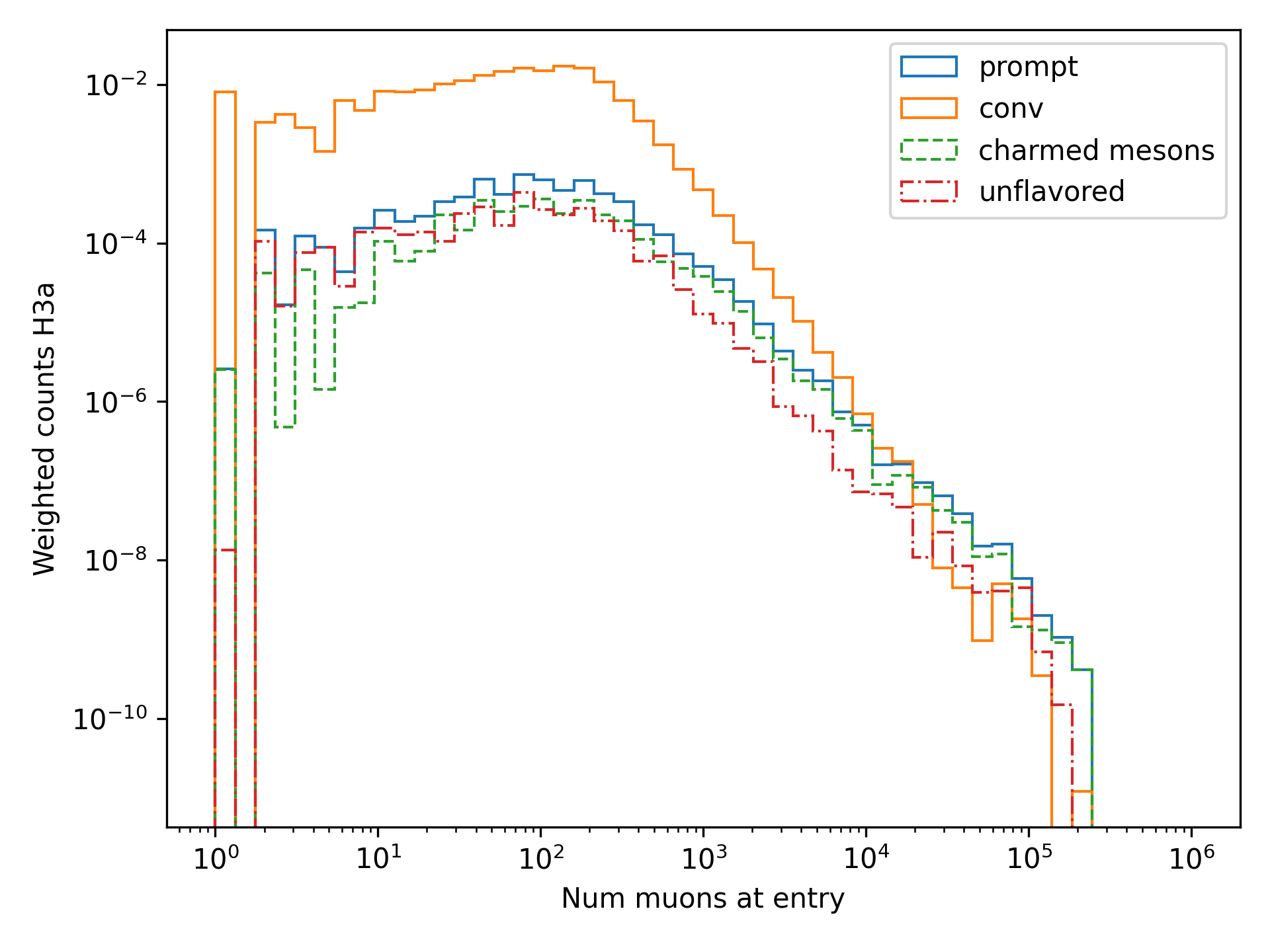
Fig. 257 : The multiplicity of charmed and unflavoured mesons is shown as a rate.
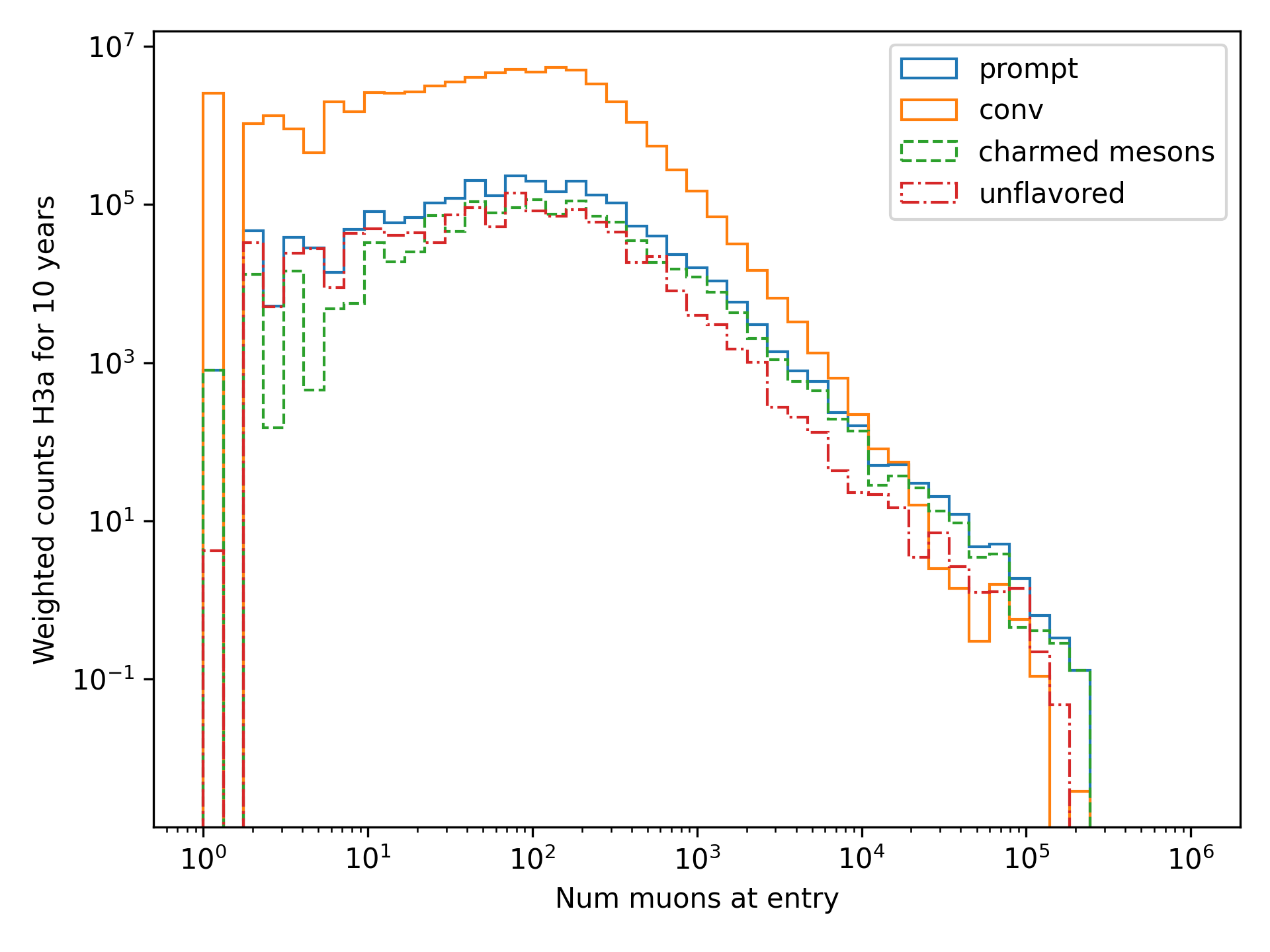
Fig. 258 : The multiplicity of charmed and unflavoured mesons is shown for the expeceted events for 10 years.
Conventional |
Charmed |
Unflavored |
|---|---|---|
pi+ |
D+ |
rho(770)0 |
K+ |
D*(2010)+ |
eta |
K(L)0 |
D0 |
omega(782) |
K(S)0 |
D*(2007)0 |
phi(1020) |
mu- |
D(s)+ |
J/psi(1S) |
D(s)*+ |
p |
|
Sigma(c)(2455)0 |
||
Lambda(c)+ |
||
Xi(c)0 |
||
Sigma(c)(2455)+ |
||
Sigma(c)(2455)++ |
||
Xi(c)+ |
Q (Lu): What atmospheric uncertainties do you include?
A: We will do our analysis for all common cosmic ray primary models, Gaisser H3a, H4a and Global Spline Fit. Since the simulation is pretty expensive, we rely on one hadronic interaction model, which will be SIBYLL 2.3d.
March 1, 2024
Q (Frank): For the angular resolution, you can show a histogram of the angular difference between the true and the reconstructed direction.
A: In principle, yes I could do that. However, we are not interested in the best angular solution here, and the resolution can be found in Fig. 35.
Q (Dave): The lateral distribution between unflavoured, charmed and conventianal should be different. Can you use machine learning to distinguish between them?
A: On the one hand, this is a stochastic process. Hence, the distributions overlap. On the other hand, the lateral distributions are on the order of \(1 \mathrm{m}\). Using the current IceCube geometry, we can not resolve this.
Q (Dave): Can you reconstruct the multiplicity with your neural networks? It would be very interesting if we can select a single muon (neutrino induced muon) from muon bundle.
A: So far, we don’t need the multiplicity for our analysis. Hence, we didn’t improve this reconstruction, but at the beginning I just trained one model to predict the multiplicity. The results are shown in Figure Fig. 332 and following. Of course, we can test the multiplicity prediction for a neutrino dataset.
Q (Dave): Can you train a network to detect/select prompt mouns?
A: This is not what we want to do. But you could for example train a network on CORSIKA simulations including prompt and on CORSIKA simulations without prompt, this depends on the hadronic interaction model. Since the entire shower profile is pretty similar, it is hard to distinguish between prompt and conventional muons. We for example also used the dynstack method to scale the prompt component up and down to test, whether the showers change to validate, that we can introduce our scaling parameter for the prompt component.
Q (Serap): You showed the network performances for the usual time window cleaning of 6000 ns and for the pulses without any cleaning. The results without cleaning seem to be better. Do you have an idea why this is the case?
A: The 6000 ns time window cleaning analyzes the weighted charge and chooses the time window with the most charged included. On the one hand, this removes successfully the after pulses, on the other hand it also removes the first pulses that arrive at the DOM. But these first pulses definitely include information about the direction and maybe also about the highest energetic muon - the leading muon. This is why the results without cleaning are better.
October 21, 2023
Q (Dave): How do you want to identify a prompt muon?
A: We do not want do identify a prompt muon. We want to measure the normalization of the prompt component.
Q (Frank): Is 20 % offset between MCEq and CORSIKA an issue?
A: These are two completely different approaches. There is no true or correct result. (see section Definitions of the prompt component)
Q (Spencer): How does the cos(theta) distribution behaves in comparison with the results of Patrick Berghaus?
A: There are similar issues. Overshoots above 0.5 and undershoots around 0.3.
Q (Anatoli): Do you set a fixed conventional normalization in your pseudo analysis? If not, to which value do you fit it?
A: No, it is not fixed. In the pseudo analysis we fit it to 0.998.
Q (Shigeru): What happens, if you use single muons?
A: For the pseudo analysis, we use the reconstructed bundle energy at entry to fit the normalization of the prompt and conventional muon flux. Here, we do not select
muons with a special leadingness. This follows from leading_bundle_energy_fraction, which shows that a high leadingness does not increase the sensitivity do detect prompt
muons. Apart from that, a single muon does not appear at high energies, there you only have muon bundles. If we select muons with a high leadingness, often referred to as
single muons, we would lose statistics and the analysis would be less sensitive.
Q (Spencer): Regarding the zenith-problem: Maybe you can estimate the impact of the magnetic field of the earth on high energy muons. Could this help to solve the problem?
A:
The radius of curvature \(R\) of a charged particle moving perpendicular to a magnetic field is given by the balance between the Lorentz force and the centripetal force:
- where
\(p\) is the momentum,
\(q\) is the charge,
\(B\) is the magnetic field strength.
For a highly relativistic muon, the momentum can be approximated by
with \(E\) the energy and \(c\) the speed of light.
Below are the calculations for both a 1 PeV muon and a 1 TeV muon.
Calculation for a 1 PeV Muon
Step 1. Convert the Muon Energy to SI Units
A muon with 1 PeV energy has
Using
we obtain
Step 2. Calculate the Momentum
For an ultra-relativistic muon,
with \(c = 3.00 \times 10^{8}\,\mathrm{m/s}\), so
Step 3. Calculate the Radius of Curvature
The muon’s charge is
and a typical Earth magnetic field is about
Substitute these values into
This radius of curvature (~67 million kilometers) is extremely large, implying that over any typical experimental or atmospheric distance the deflection of a 1 PeV muon by the Earth’s magnetic field is negligible.
Calculation for a 1 TeV Muon
Step 1. Convert the Muon Energy to SI Units
A muon with 1 TeV energy has
so
Step 2. Calculate the Momentum
Again, using
with \(c = 3.00 \times 10^{8}\,\mathrm{m/s}\), we have
Step 3. Calculate the Radius of Curvature
Using the same charge and magnetic field:
the radius is
This gives a radius of curvature of roughly \(6.67 \times 10^{7}\,\mathrm{m}\) (or about 66,700 kilometers). Although this is smaller than the 1 PeV case by a factor of 1000, it is still extremely large compared to typical distances encountered in experiments or in the atmosphere.
Interpretation
In both cases, the large radius of curvature means that the deflection of the muon due to the Earth’s magnetic field is negligible over the scales of most experiments. For a 1 PeV muon the radius is on the order of \(10^{10}\,\mathrm{m}\), and for a 1 TeV muon it is on the order of \(10^{7}\,\mathrm{m}\).
Q (Spencer): How large are the uncertainties on the conventional component (pion/kaon production)?
A: TODO
Q (Spencer): How large is the background that we expect (astrophysical neutrinos, atmospheric neutrinos)? If we are able to distinguish between a single muon and a muon bundle, we can remove neutrino induced background muons.
A: To estimate the neutrino background, the bundle energy at entry is shown in Fig. 259. The NuGen background includes both atmospheric and astrophysical neutrinos. At the highest energies of \(10 \mathrm{PeV}\), it’s on the order of a few percent. It decreases to below \(1 \mathrm{%}\) at lower energies. Regarding the distinction between single muons and muon bundles, I made some very preliminary studies. It seems to be quite promising, but it definitely needs more investigation. Since I used some assumptions, uploading the plots might be confusing. I can provide some plots upon request.
Fig. 259 : Bundle energy at entry is shown to estimate the neutrion background. The NuGen background in purple includes both atmospheric and astrophysical neutrinos. The atmospheric neutrinos are estimated using MCEq and GaisserH3a. The astrophysical neutrinos are calculated with \(\gamma = 2.6\) with a normalization of \(n = 1.5\).
September 29, 2023
Q (?): In the simulation you remove the electromagnetic shower component. Thus, you also remove some muons. How large is the impact of this to your analysis?`
A: We used CORSIKA 8 to estimate the impact of the electromagnetic shower component on the produced muons. For a 500 PeV proton shower, the total amount of muon-energy per shower is about 4.8 %. For the large-scale simulation we will simulate the EM component, if the simulation of the EM component is feasible. This impact was investigated by Jean-Marco and is shown in Fig. 260 and Fig. 261.
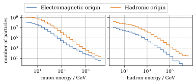
Fig. 260 : CORSIKA 8 was used to simulate 500 PeV proton showers to estimate the impact of the electromagnetic shower component.
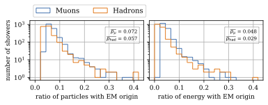
Fig. 261 : The ratio of the number of muons and the energy of the muons is shown for 500 PeV proton showers. On average, 4.8 % of the energy is carried by muons originating from the electromagnetic shower component.
Q (?): Your prompt definition is: parent is not pion or kaon. The definiton in MCEq divides prompt and conventional by a minimum decay length of 0.123 cm. Is there a difference?
A: The “lifetime” definition is similar, as it includes every particle with a lifetime which is greater than ten times the lifetime of the D0 as conventional and the rest as prompt. This is the definition of prompt used inside MCEq, and the lifetime limit corresponds to a decay length of approximately 1.2 cm. Considering all particles in CORSIKA7, these are the photon, electron, muon and neutrino from the fundamental particles. Of these none can decay into a muon. But in CORSIKA, a muon can be listed as the parent of a muon. These would then be considered to belong to the conventional component. The hadrons below the lifetime limit are pion, K±, KL, KS, which are exactly the pion and kaons from the pion-kaon definition. The Baryons below the lifetime limit are 𝑝, 𝑛, 𝛬, 𝛴±, 𝛯0, 𝛯±, of these only the proton and the neutron can not decay into a muon. These baryons and the muon is the only difference compared to the pion-kaon definition of prompt. These particles do not seem to contribute much to the flux, as both of the definitions produce nearly identical results, see section Definitions of the prompt component.
Q (Agnieszka): How do you plan to reconstruct the leading muon energy?
A: For the reconstruction of the leading muon energy, we use a convolutional neural network. Further details can be found in the Reconstructions section of this wiki.
Q (Jakob): In your pseudo analysis you used a poisson likelihood. Do you want to add limited statistics to your likelihood?
A: Yes, we do want use the Say likelihood. Apart from that, for the real analysis we will probably switch to the tool NNMFit. This is already known in IceCube and in our first test it seems to work for us as well. Thus, we can avoid code duplication. In addition, the tools is able to perform fits with multiple datasets. In the future, this helps do to a combined fit with a atmospheric muon and neutrino dataset.
Q (Jakob?): What is the impact of limited MC statistics on your analysis currently?
A: As you can see in the section New CORSIKA extended history simulations, we have a quite sufficient statistics for high energies, but to little statistics for low energies. Hence, especially the low energy events are oversampled in the pseudo dataset. For the real analysis, we will simulate a new datasets with more statistics to reach statistical uncertainties lower than our systematic uncertainties. But to estimate our systematic uncertainties, we already need more statistics.