Selection

The starting point for the selection is level 2. The rate for all events depends on the underlying primary model. For the common primary models H3a, H4a, GST and GSF, the rates on level2 are shown in Table 1. For example, using H3a, the number of total events per run (8h) can be estimated, which is more than 83 Mio. events. A single run is processed by a single processor unit. Assuming an average processing time of 1 second per event, the runtime per run would be longer than 23k hours, which is not feasible. Hence, a fast selection is necessary to remove statistics. As presented in Fig. 1, the prompt muon flux becomes more dominant towards higher energies, and it is suppressed by orders of magnitude at lower energies. Thus, low energy muons need to be removed.

Table 1 Rates on level 2 before applying any filter for different primary models based on simulations 22774-22778 and 22875.

Model	H3a	H4a	GST	GSF
Level2 rate / Hz	2887.86	2956.16	2725.19	2941.80

In a first step, several filters are investigated in regard to the energy of the leading muon at surface and the cosine zenith angle. The muon filter results as the best choice, defining Level 3. Afterwards, a cut on the bundle energy at surface is applied to remove more low energy events, and DNN reconstructions for several properties are added. This defines Level 4. In level 5, quality cuts are applied to improve the data-MC agreement. At last, events with a minimum leadingness are selected. This is the Final Level. Table 2 presents a summary of the entire selection.

Table 2 Summary of the entire leading muon selection.

Level	Level 3	Level 4	Level 5	Final Level
Selection	MuonFilter	Bundle energy at surface > 500 TeV	Data-MC quality cuts	Leadingness > 0.4

The following sections describe the selection steps in detail.

Level 3

Filters

The detection of atmospheric prompt muons requires high energy events. Thus, five different filters focusing on high energy events are tested to get rid of low energy events while keeping as many as possible high energy events. Table 3 shows the fraction of passed events for different energy bins, filters and weightings.

Fig. 27 : Investigating the impact of several filters on level 2 for the leading muon energy at surface for H3a.

Fig. 28 : Investigating the impact of several filters on level 2 for the cosine of the primary zenith angle for H3a.

Table 3 Fraction of events passed filters for different energy bins and weightings. Muon energy at surface is considered.

Filter	10 TeV < E < 100 TeV	100 TeV < E < 1 PeV	1 PeV < E < 10 PeV	10 PeV < E < 100 PeV	All energies
MuonFilter, GaisserH3a	2.8e-01	7.8e-01	8.3e-01	1.0e+00	1.2e-02
OnlineL2Filter, GaisserH3a	1.2e-01	6.3e-01	7.9e-01	8.6e-01	2.9e-03
HighQFilter, GaisserH3a	3.0e-02	2.8e-01	5.1e-01	6.4e-01	5.1e-04
EHEAlertFilter, GaisserH3a	0.0e+00	1.8e-07	2.0e-05	0.0e+00	4.6e-12
EHEAlertFilterHB, GaisserH3a	2.9e-06	8.3e-04	3.2e-02	2.1e-01	4.4e-08
MuonFilter, GlobalSplineFit5Comp	2.7e-01	7.8e-01	7.6e-01	1.0e+00	1.2e-02
OnlineL2Filter, GlobalSplineFit5Comp	1.2e-01	6.2e-01	7.3e-01	9.5e-01	2.6e-03
HighQFilter, GlobalSplineFit5Comp	2.6e-02	2.7e-01	5.6e-01	6.1e-01	4.1e-04
EHEAlertFilter, GlobalSplineFit5Comp	0.0e+00	9.7e-08	2.4e-05	0.0e+00	3.3e-12
EHEAlertFilterHB, GlobalSplineFit5Comp	1.7e-06	4.0e-04	2.7e-02	3.0e-01	2.5e-08

In the final analysis, the lower bound of the muon energy at surface is 10 TeV. As presented in Table 3, the MuonFilter rejects in total 98.8% of the events, but keeps the most events for the 4 energy intervals between 10 TeV and 100 PeV. Regarding the cosine zenith distribution, the HighQFilter removes more horizontal events than the MuonFilter. This is caused by the fact, that horizontal, high energy events travel through a large amount of ice and thus have a large amount of energy losses. In the detector, they are not able to pass the high-charge filter, since they arrive with a lower energy. However, since we want to reconstruct the muon energy at surface, we want to keep these events. Hence, the MuonFilter is used.

The rates after the application of the MuonFilter are shown in Table 4. This results in a runtime of 150h per run with a processing time of 1s per event. This is still too long.

Table 4 Rates on Level 3 after applying the muon filter for different primary models.

Model	H3a	H4a	GST	GSF
Level 3 / Hz	18.43	18.83	17.41	17.85

Level 4

To further reduce the number of events in the low energy region, a cut on the bundle energy at surface is applied. For this, the efficiency as a ratio of the number of events before and after the cut is calculated. Here, two cuts are compared: a cut of \(200\,\mathrm{TeV}\) and a cut of \(500\,\mathrm{TeV}\). The 200 TeV cut is motivated by a target rate roughly about \(125\,\mathrm{mHz}\), which would refer to a runtime of 1h per run with a processing time of 1s per event for an 8h run. As shown below, for H3a, the rate is about \(176\,\mathrm{mHz}\) for the 200 TeV cut. Since this cut still keeps almost all muons at surface above 500 TeV, a cut of 500 TeV is also investigated. This cut reduces the rate to \(22\,\mathrm{mHz}\) for H3a, and it also keeps lots of events in the high energy region.

In the following, 3 plots are shown which present the efficiency for the leading muon energy at surface and detector entry and for the primary energy.

– Primary Energy –

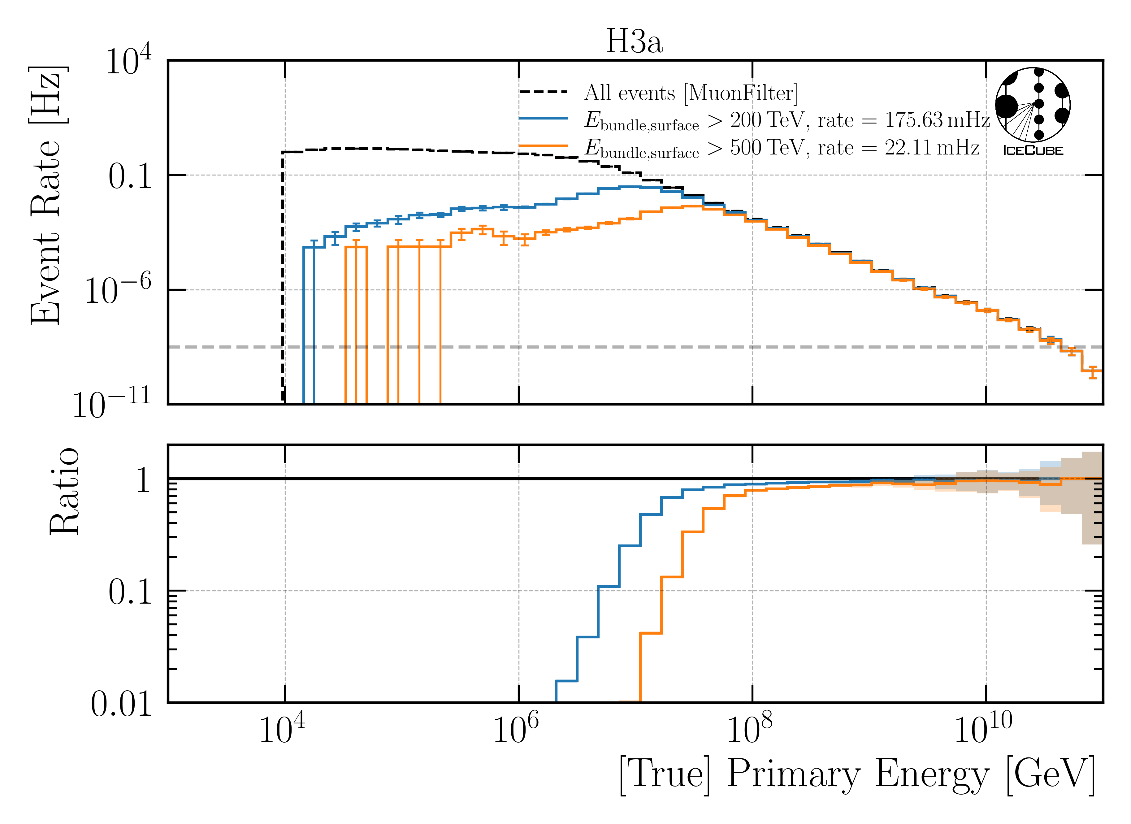
Fig. 29 : Efficiency for the primary energy for H3a.

– Leading Muon Energy at Surface –

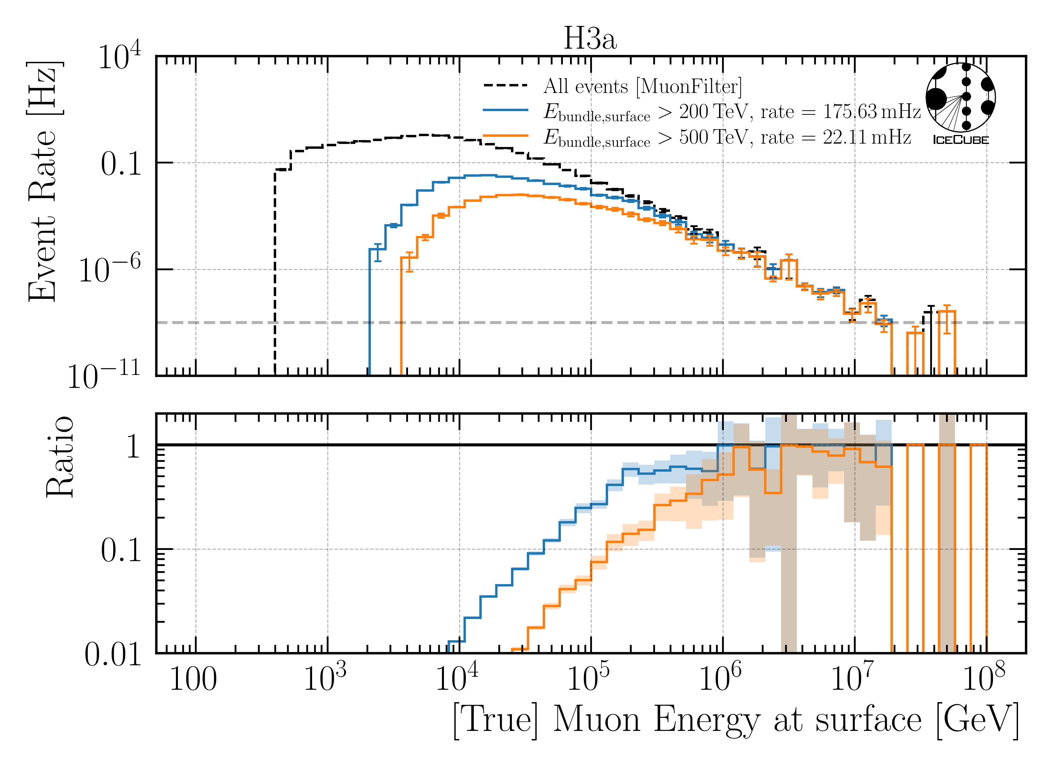
Fig. 30 : Efficiency for the leading muon energy at surface for H3a.

– Leading Muon Energy at Entry –

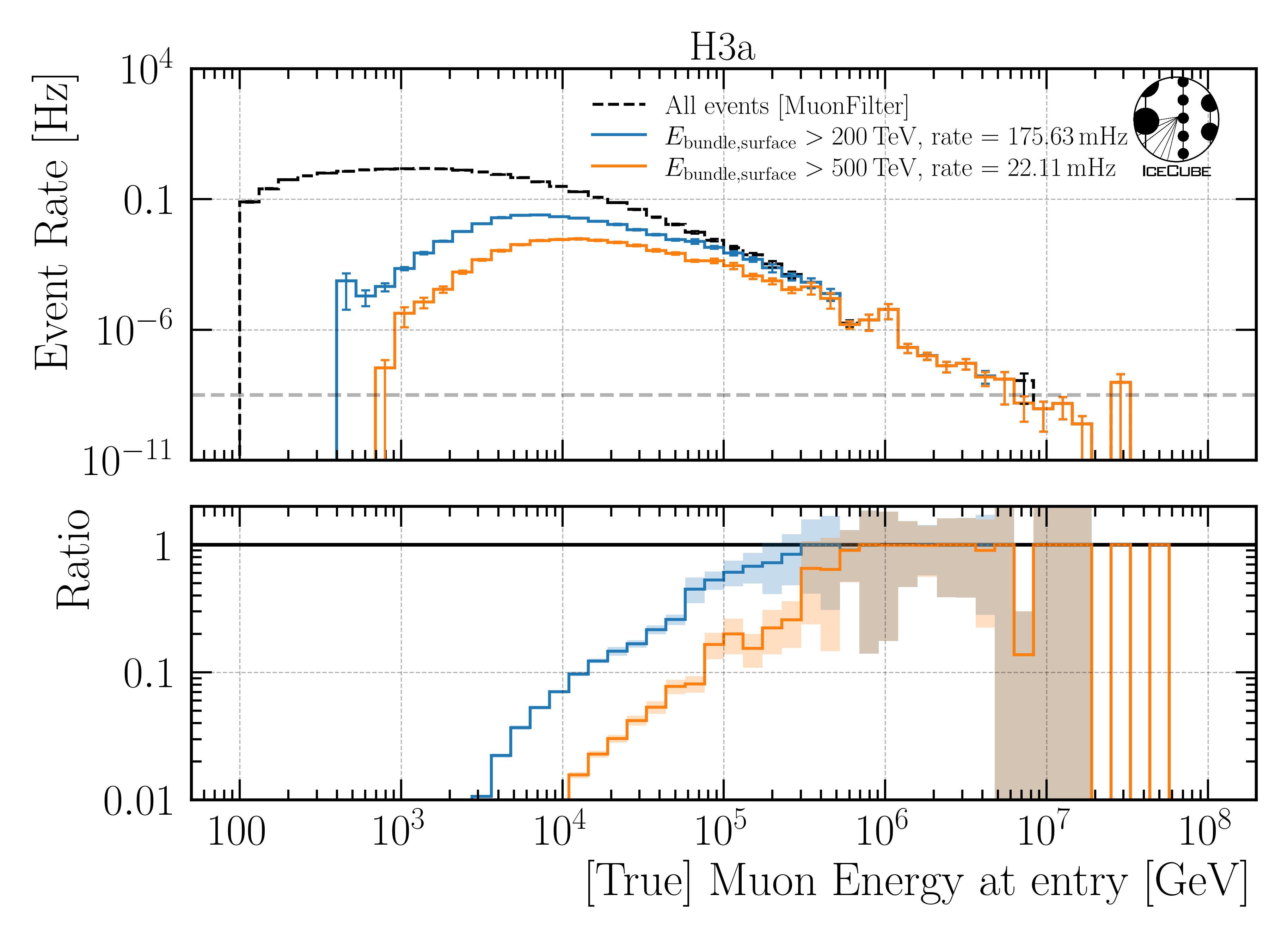
Fig. 31 : Efficiency for the leading muon energy at entry for H3a.

In the following, the remaining rate after applying the MuonFilter and a bundle energy cut at surface of \(200\,\mathrm{TeV}\) is shown in Table 5, and for a cut of \(500\,\mathrm{TeV}\) in Table 6.

Table 5 Rates on level 3 after applying the muon filter and a \(200\,\mathrm{TeV}\) bundle energy cut at surface for different primary models.

Model	H3a	H4a	GST	GSF	Exp
Level 4 (test) / mHz	173.4	171.9	164.3	124.1	158.2

Table 6 Rates on level 3 after applying the muon filter and a \(500\,\mathrm{TeV}\) bundle energy cut at surface for different primary models.

Model	H3a	H4a	GST	GSF	Exp
Level 4 / mHz	21.62	21.09	20.92	14.07	18.55

For our level 4, we apply the MuonFilter and a cut of \(500\,\mathrm{TeV}\) on the bundle energy at surface. The remaining rate is \(21.62\,\mathrm{mHz}\). The pre-cut network DeepLearningReco_precut_surface_bundle_energy_3inputs_6ms_01 is used for this cut.

Furthermore, the DNN reconstructions mentioned in the reconstruction section are added at this stage. For this, the following networks are added:

• DeepLearningReco_direction_9inputs_6ms_medium_02_03 reconstructs: zenith and azimuth of the leading muon

• DeepLearningReco_leading_bundle_surface_leading_bundle_energy_OC_inputs9_6ms_large_log_02 reconstructs: bundle/leading muon energy at surface/detector entry

• DeepLearningReco_track_geometry_9inputs_6ms_medium_01 reconstructs: propagation length, entry and center position

Already added in step 3:

• DeepLearningReco_precut_surface_bundle_energy_3inputs_6ms_01 reconstructs: bundle energy at surface

In Table 7, the runtimes for the DNN reconstructions are shown. The preprocessing time is needed to create the input features for the DNNs based on the input pulses. The preprocessing time of the precut network is faster, since only 3 input features instead of 9 features are calculated. The CPU and GPU times are the runtimes needed to apply the DNNs on the respective device.

Table 7 DNN reconstruction runtimes

Network	Preprocessing / ms	CPU / ms	GPU / ms
Direction	22 ± 20	106 ± 42	5 ± 38
Energy	22 ± 20	144 ± 56	3 ± 13
Track geometry	22 ± 20	106 ± 42	3 ± 10
precut	1 ± 1	11 ± 1	7 ± 4

Level 5

Cuts presented here are based on the plots in Data-MC.

For level 5, quality cuts are performed to improve the data-MC agreement. Furthermore, some additional cuts are performed to remove neutrino background events. For the reconstruction of the bundle energy, the network learns, that if an event is entering the detector from the horizon, it must be very high-energetic because it was able to pass the Earth. Cutting away events from the horizon removes these neutrino events. The third category of cuts is based on the uncertainty estimation provided by the DNN reconstructions as mentioned before.

In Table 8, the cuts to improve data-MC based on the detector geometry are presented. In Table 9, the cuts to remove neutrino background events are shown. Table 10 shows the cuts based on the uncertainty estimation.

Table 8 Containment Cuts

Containment Cuts	>	<
length in detector	1000 m	2000 m
entry pos x, y	-750 m	750 m
entry pos z	-500 m	750 m
center pos x, y	-550 m	550 m
center pos z	-650 m	650 m

Table 9 Neutrino Cuts

Neutrino Cuts	>	<
cos(zenith)	0.2
length	5000 m	15000 m

Table 10 Uncertainty Cuts

Uncertainty Cuts	<
bundle energy at entry	0.9 log10(GeV)
bundle energy at surface	2.0 log10(GeV)
zenith	0.1 rad
azimuth	0.2 rad
entry pos x, y, z	42 m
center pos x, y, z	50 m
entry pos time	200 ns
center pos time	600 ns
length in detector	160 m
length	2000 m

In Table 11, the rates after applying the muon filter, the \(500\,\mathrm{TeV}\) bundle energy cut at surface and the quality cuts for different primary models are shown.

Table 11 Rates on level 5 after applying the muon filter, the \(500\,\mathrm{TeV}\) bundle energy cut at surface and the quality cuts for different primary models.

Model	H3a	H4a	GST	GSF	Exp
Level 5 / mHz	15.16	14.76	14.79	9.68	12.36

Final Level

At last, a cut on the leadingness (ratio between most energetic muon and total bundle energy) is applied to improve the data-MC agreement of the proxy variable for the unfolding, the leading muon energy at entry. It is required, that the most energetic muon carries at least 40% of the total energy of the muon bundle. The data-MC agreement for the proxy variable used to unfold the atmospheric muon flux is presented on the burnsample dataset in Fig. 32. For all four different primary cosmic-ray models, the data agree with the MC prediction. A different slope is visible for the weightings, however, this is expected. The different primary cosmic-ray models predict different fluxes and thus, different spectral indices. Per definition, this effect propagates from the primary particle to the final reconstructed muon. Hence, a difference between the models is expected.

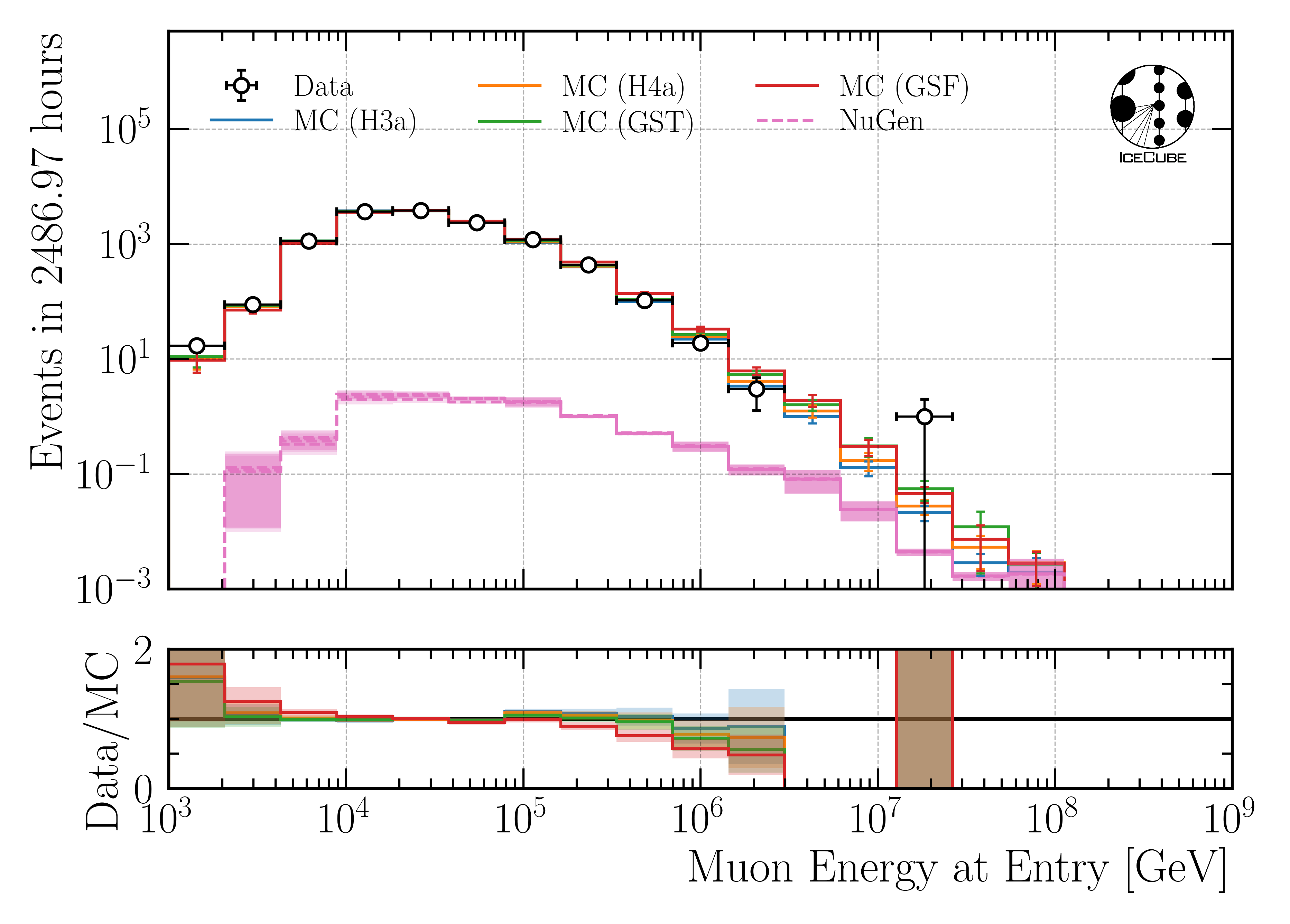
Fig. 32 : Proxy variable utilized to unfold the atmospheric muon flux at surface on the final selection stage.