One Page Summary
This page includes a summary of the entire analysis chain. This helps to get a quick overview of the analysis.
Analysis Goal
The goal of this analysis is an unfolding of the atmospheric muon flux in the energy from 10 TeV to about 10 PeV using the IceCube in-ice array. This enables to become sensitive to heavy mesons decaying in the atmosphere, referred to as prompt (see Fig. 12).
Prompt Definition
A muon is categorized as prompt or conventional depending on its parent particle (see Prompt Definition).
Conventional: muon parent is a pion or a kaon
Prompt: all other parent particles
New CORSIKA EHIST Simulation
For the analysis, new CORSIKA simulations with the extended history option are generated with IceProd. This option allows to get the information of the muon parent to classify a muon as prompt or conventional. The datasets were created with the hadronic interaction model SIBYLL 2.3d. More information are stored at New CORSIKA Simulation.
CNN Reconstructions
All reconstructions uitilized in this analysis are machine learning based using the dnn_reco framework. The networks are trained on several older CORSIKA simulation datasets. In total, 4 different networks are trained and used in the analysis. One network is used to perform a quick pre-cut to remove lower energetic events. The other three networks reconstruct properties like muon energies, directions and detector geometries (entry points etc.). The networks also predict an uncertainty on the reconstructed property. In the figure below, the proxy variable for the unfolding (leading muon energy at detector entry ) is shown.
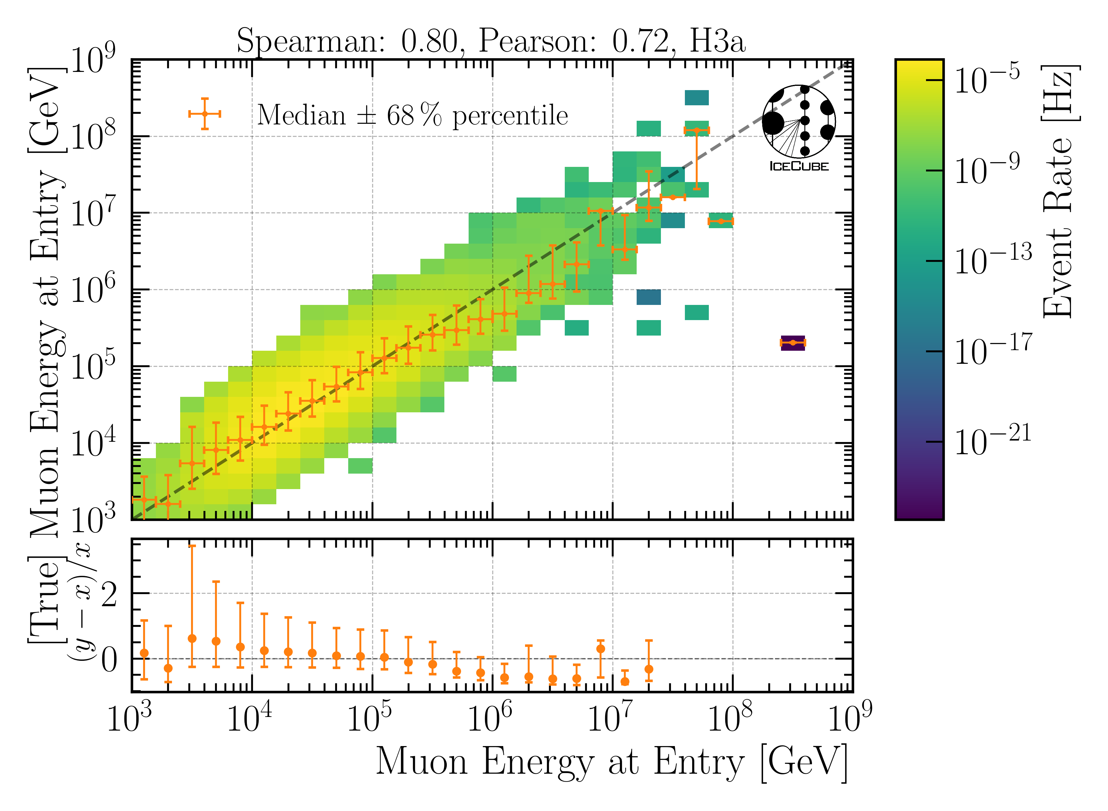
Fig. 1 : Performance of the leading muon energy reconstruction on the final selection level. This variable is used as a proxy to unfold the atmospheric muon flux at surface.
Details are provided at CNN reconstructions.
Selection
This analysis is based on a new selection performed within the scope of this analysis. Since the goal is an unfolding of the atmospheric muon flux for energies above 10 TeV, the idea is to select high-energetic muons. This is reached by several selection steps, labeled as Level3, Level4, Level5 and FinalLevel.
Level3: Applying the muon filter to select muons
Level4: Use the pre-cut network to remove events with a muon bundle energy at surface with below 500 TeV
Level5: Use the other networks to perform several data-MC comparisons for the direction, detector entry point, closest approach point to the center, propagation length, the predicted uncertainties, etc. A bunch of cuts is performed to improve the data-MC agreement for several properties to select well reconstructed muons.
FinalLevel: To improve the data-MC agreement on the energy estimator used in this analysis – the reconstructed energy of the most energetic muon in the muon bundle (leading muon) – it is required that the leading muon carries at least 40% of the entire muon bundle energy at the entry point of the detector.
The data-MC agreement of the energy proxy at the final selection stage used for the unfolding in this analysis is shown in Fig. 2.
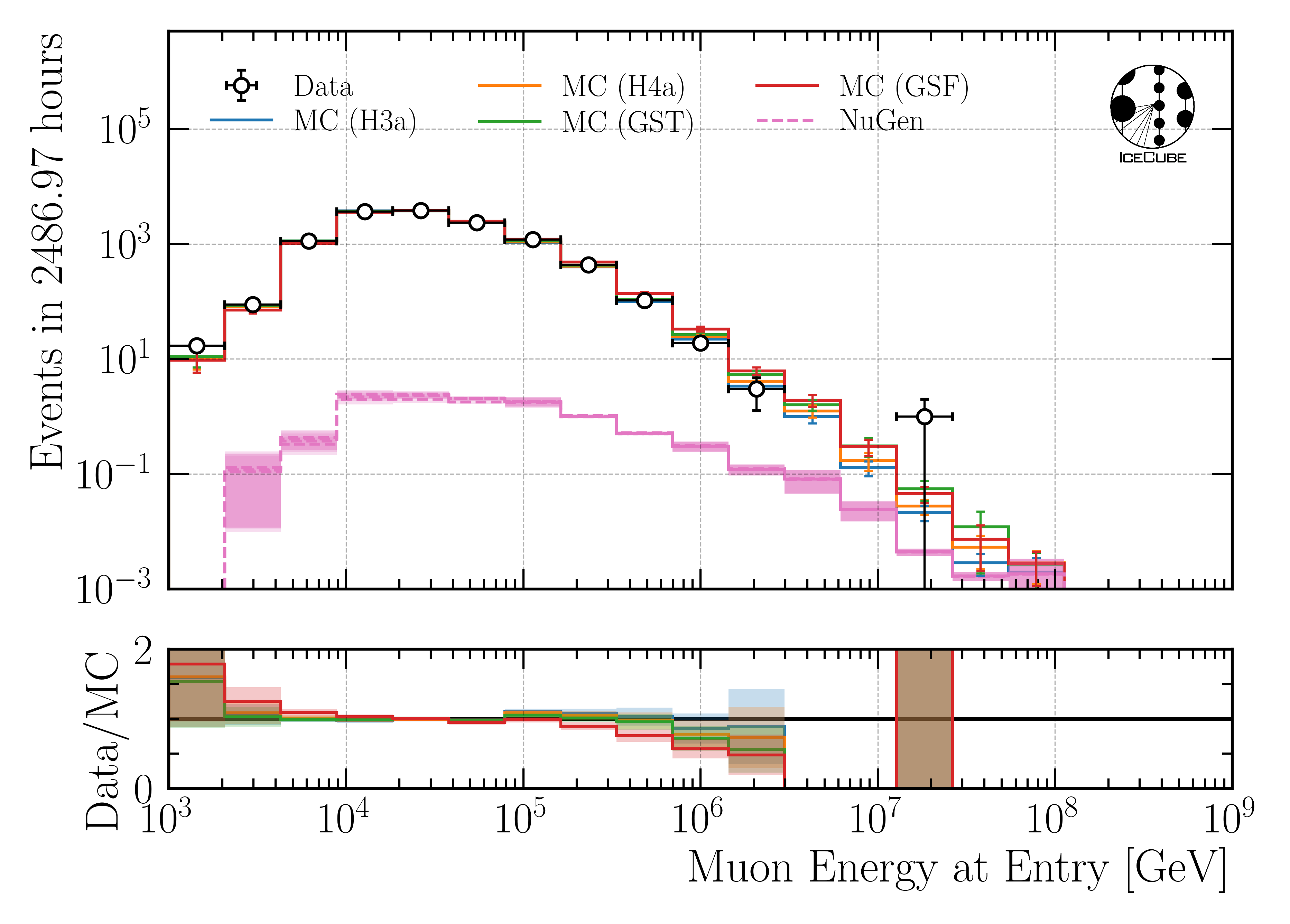
Fig. 2 : Proxy variable utilized to unfold the atmospheric muon flux at surface on the final selection stage.
Detailed information of the selection can be found at Selection. The data-MC checks on the different selection levels are provided at Data-MC Level 4, Data-MC Level 5 and Data-MC Final Level.
Unfolding
The distribution of a measured quantity \(g(y)\) is connected to the true physical distribution \(f(x)\) via the detector response \(A(x,y)\) according to the convolution integral
This is referred to as the Fredholm integral equation of the first kind. The additional term \(b(y)\) represents some bias, which originates form contributions to the measurement that are considered as background. Since the selected sample is assumed to have a sufficiently high purity, the bias will be neglected in the following. The detector response function \(A(x,y)\) describes the whole detection procedure. It depends on the physical truth and has to be determined from Monte Carlo simulations. Details on the unfolding can be found at Unfolding paragraph.
Systematic uncertainties are considered in the detector response as well by modeling the effect of the five in-ice systematics on the effective bin count. More information on the systematics can be found at Systematics paragraph.
In the following, the measured quantity is called proxy and the true physical quantity target.
Proxy–Target Correlation
In this analysis, the leading muon energy at the detector entry point is used as a proxy to unfold the atmospheric muon flux at surface. The correlation is presented in Fig. 3.
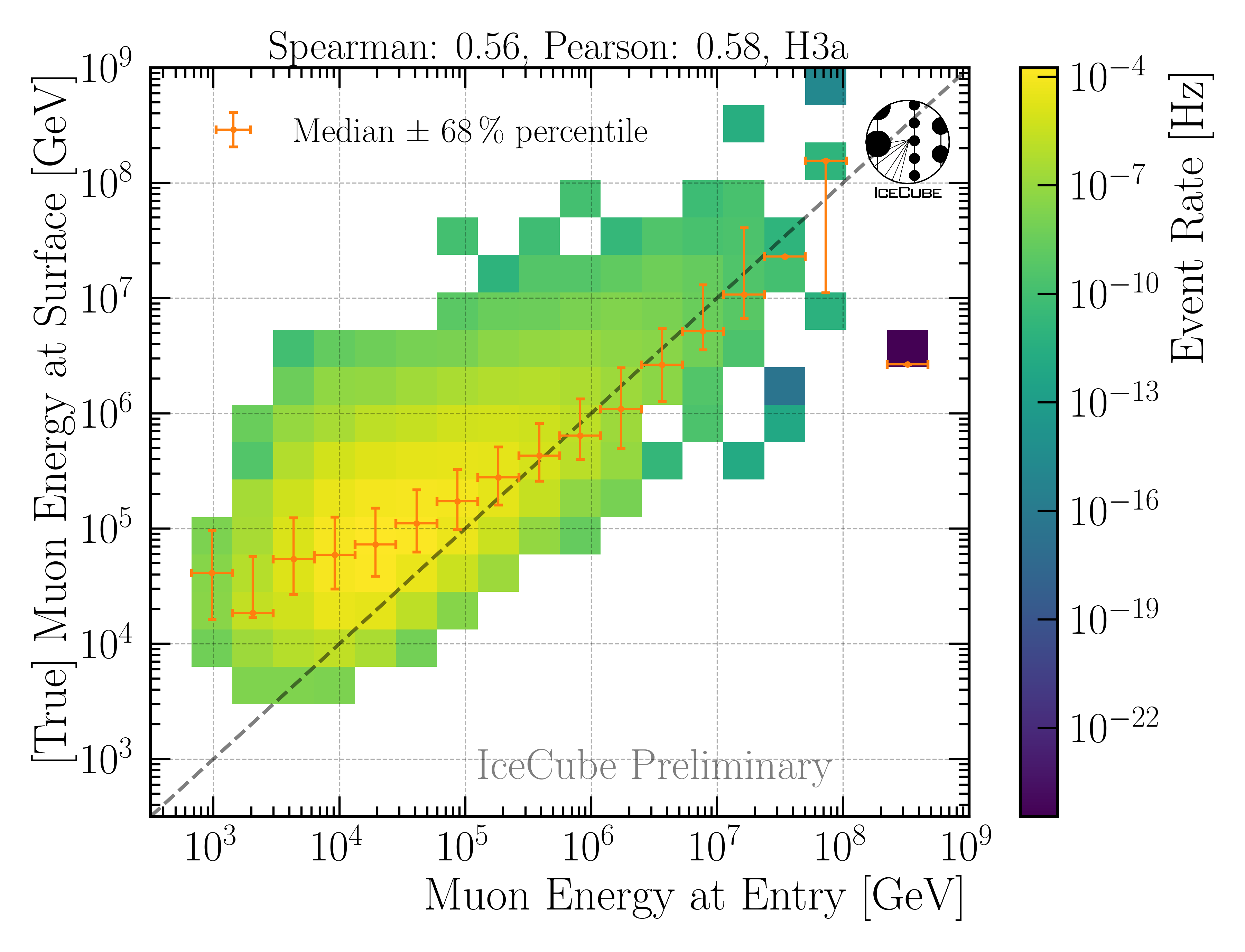
Fig. 3 : Proxy variable for unfolding. Here, the muon energy of the leading muon at entry is used. The target is the leading muon energy at surface.
Regularization strength
To minimize unphysical fluctuations in the unfolded result, a regularization is applied using Tikhonov regularization of order 2. The strength of the regularization is determined by scanning the global correlation coefficient \(\rho\) as a function of the regularization parameter tau. Here, it is
where V is the covariance matrix of the unfolded distribution, with i and j being the indices of the unfolding bins. The optimal regularization strength tau is found by minimizing the global correlation, as presented in Fig. 4. The correlation curve is smooth and a minimum can be found easily.
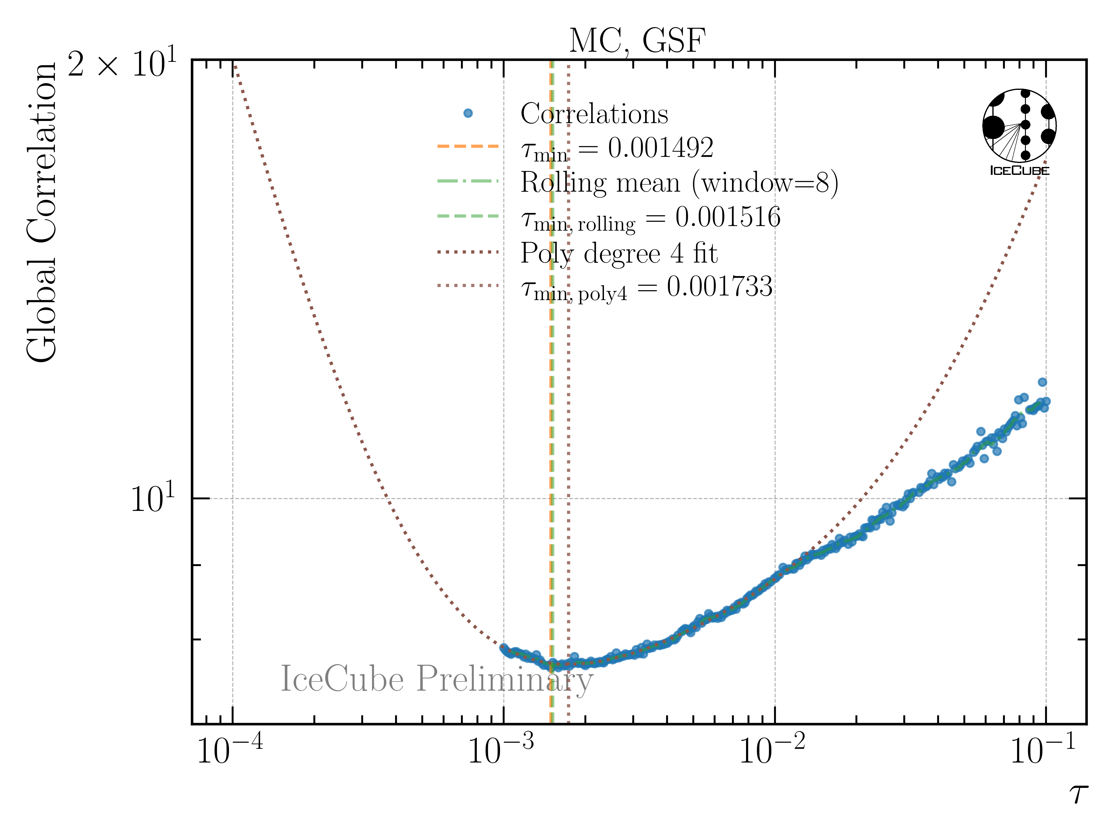
Fig. 4 : Global correlation as a function of the regularization parameter tau. The unfolding algorithm is trained on H3a and tested on GSF.
The unfolding is only accepted, if the minimization using minuit is successful, otherwise the point is discarded. To avoid fluctuations in the distribution, a rolling average and a polynomial fit around the expected minimum is used to determine the optimal tau value. In Fig. 5, the global correlation is shown, when the unfolding algorithm is both trained and tested on H3a. Here, the curve is less smooth, however, all three methods determine a similar optimal tau value.
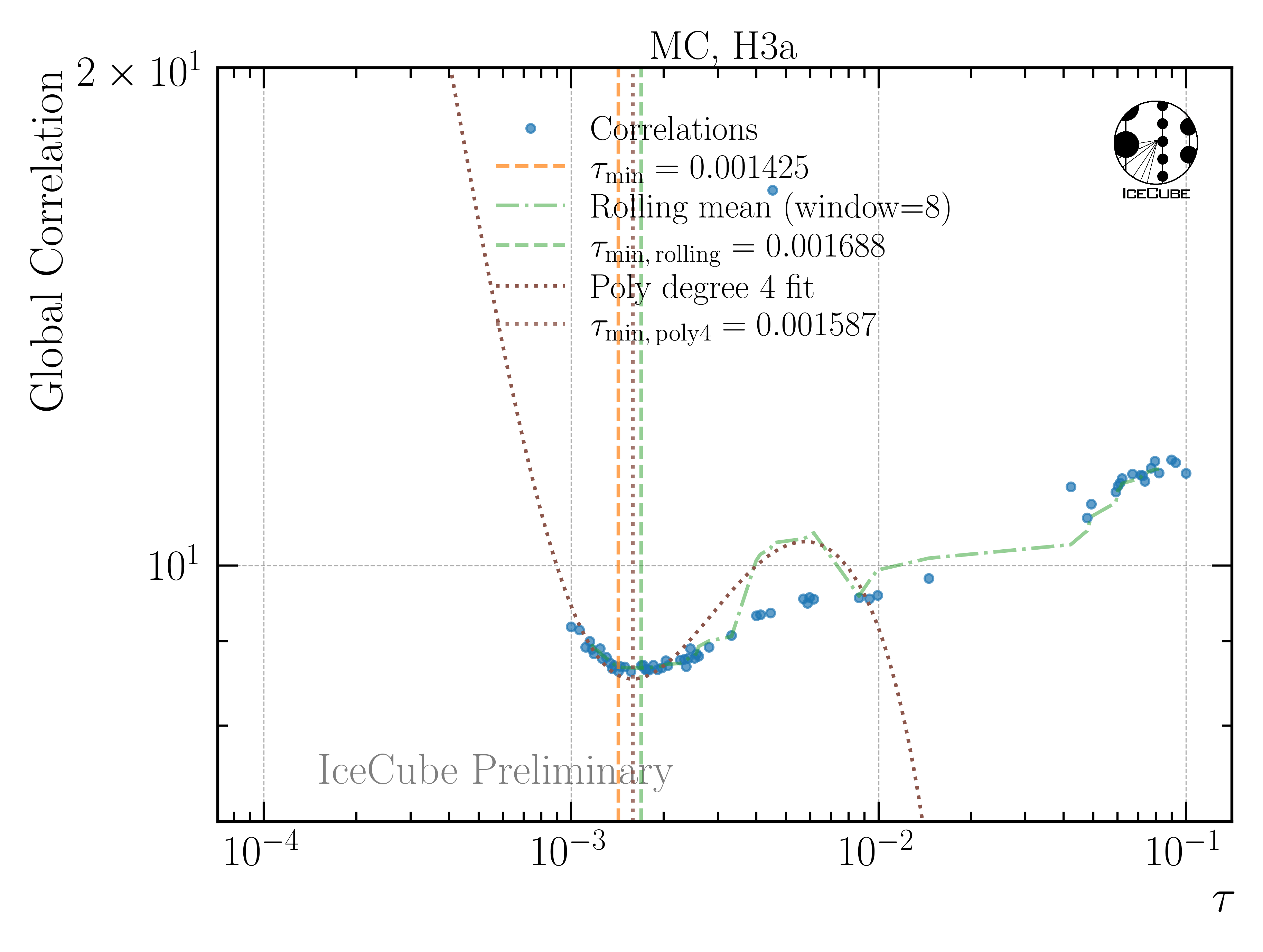
Fig. 5 : Global correlation as a function of the regularization parameter tau. The unfolding algorithm is trained and tested on H3a.
Effective Area
The effective area \(A_{\mathrm{eff}}\) describes the detector acceptance and is defined as
where \(N_{\mathrm{detected}}\) is the number of detected events after all selection cuts, \(N_{\mathrm{generated}}\) is the number of generated events in the simulation, and \(A_{\mathrm{gen}}\) is the generation area. The effective area is shown for the burnsample in Fig. 6.
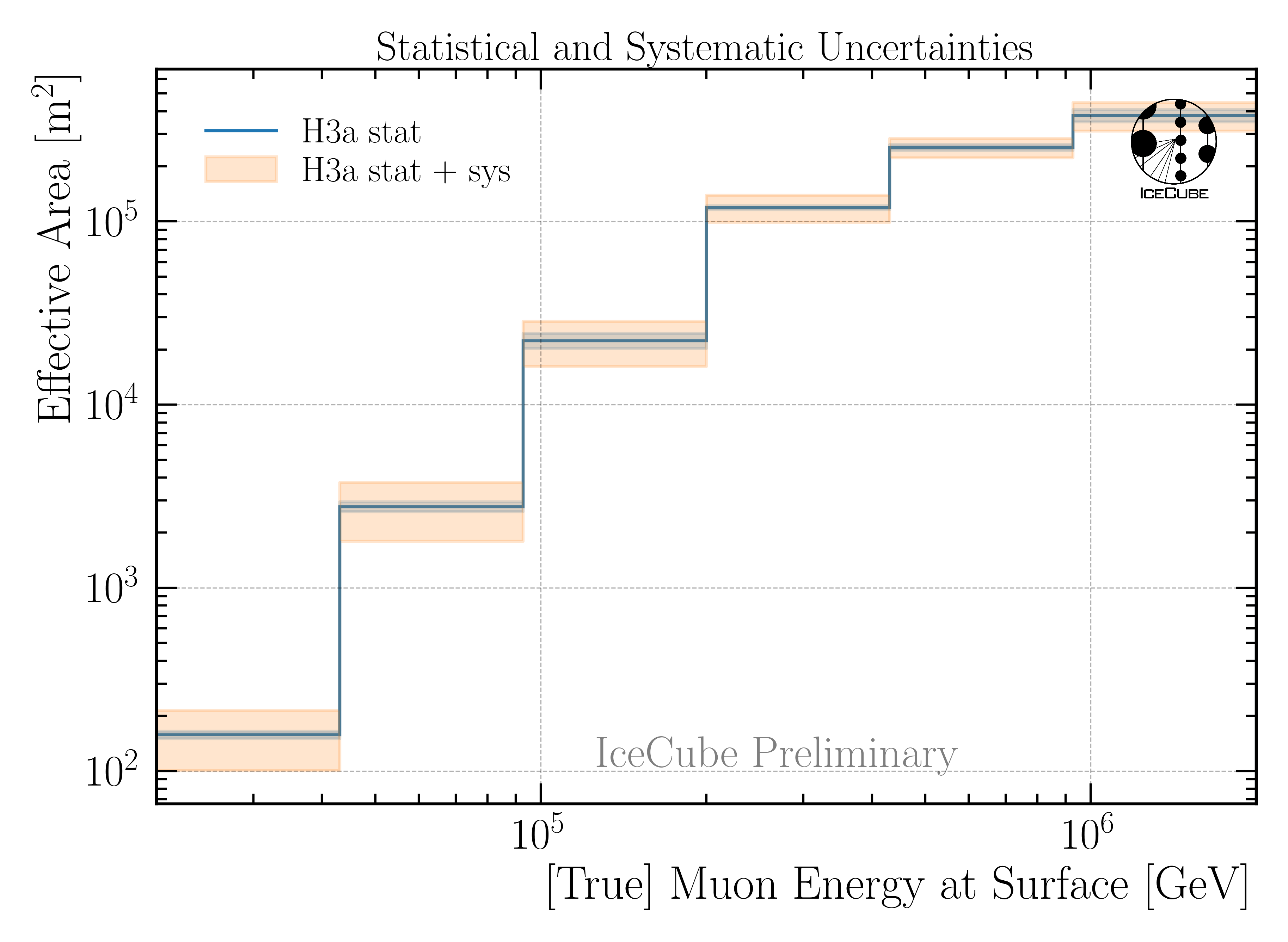
Fig. 6 : The effective area is presented as a function of the muon energy at surface. Statistical uncertainties are calculated with the weights. The systematic uncertainties result from the variations in the effective area. This is shown for the burnsample binning.
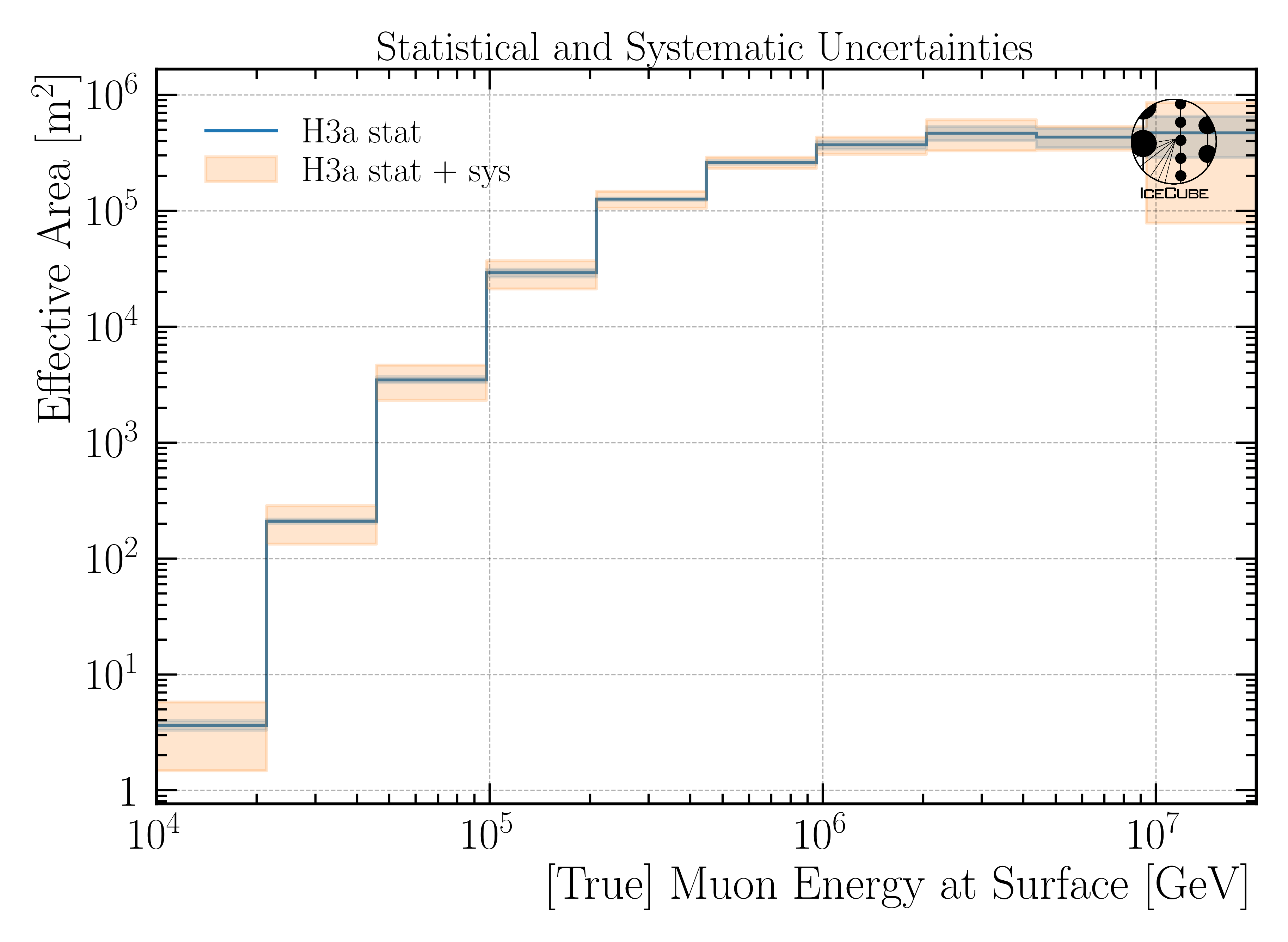
For the full 12 years sample, the effective area is shown in effective_area_fullsample_1.
More information on the effective area and the corresponding systematic uncertainties are described in Unfolding/Effective Area. This is done analogue to the analysis of stopping muons by Lucas Witthaus (see Stopping muons wiki).
Burnsample Unfolding
The burnsample unfolding has been presented at the ICRC and the proceedings is available here: Unfolding the Atmospheric Muon Flux with IceCube: Investigating Stopping Muons and High-Energy Prompt Contributions. Here, more information can be found at Burnsample Unfolding.
The final result is presented in Fig. 7.
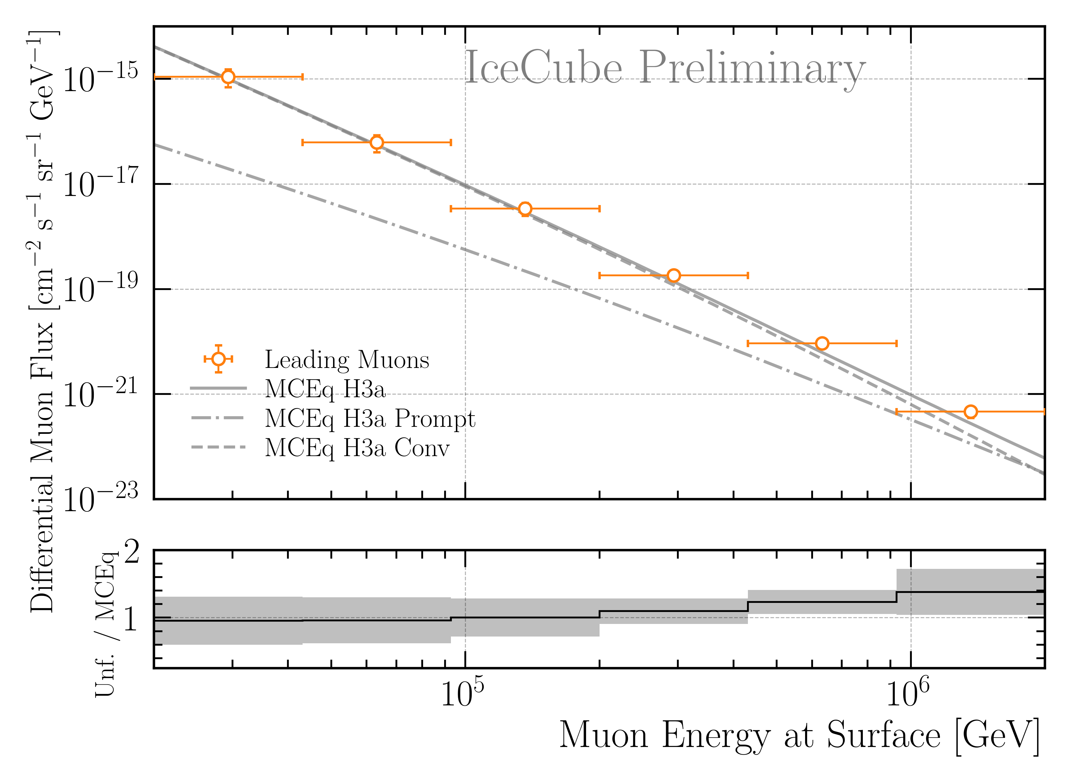
Fig. 7 : Unfolded muon flux at surface using the burnsample data with \(2487\,\mathrm{h}\) of IceCube data. The unfolding is performed with tau=0.0029. The uncertainties are derived from the inverse of the Hessian matrix obtained in the Minuit fit and are further expanded to include the systematic variations of the effective area. The unfolded result is compared to predictions from MCEq using H3a, and SIBYLL 2.3c.
Full Sample Unfolding
For the full sample, 12 years of data IC86 will be used. The unfolding is performed analogue to the burnsample unfolding. However, the uncertainties are treated slightly different.
The total uncertainty on the unfolded flux is given by
Here, \(\sigma_{\text{minuit}}\) is derived from the inverse of the Hessian matrix obtained in the Minuit fit. This fit also includes the 5 in-ice systematics. \(\sigma_{\text{Aeff,stat}}\) is the statistical uncertainty on the effective area, and \(\sigma_{\text{unf-bias}}\) is the uncertainty due to a possible unfolding bias. This bias is presented in Fig. 8.
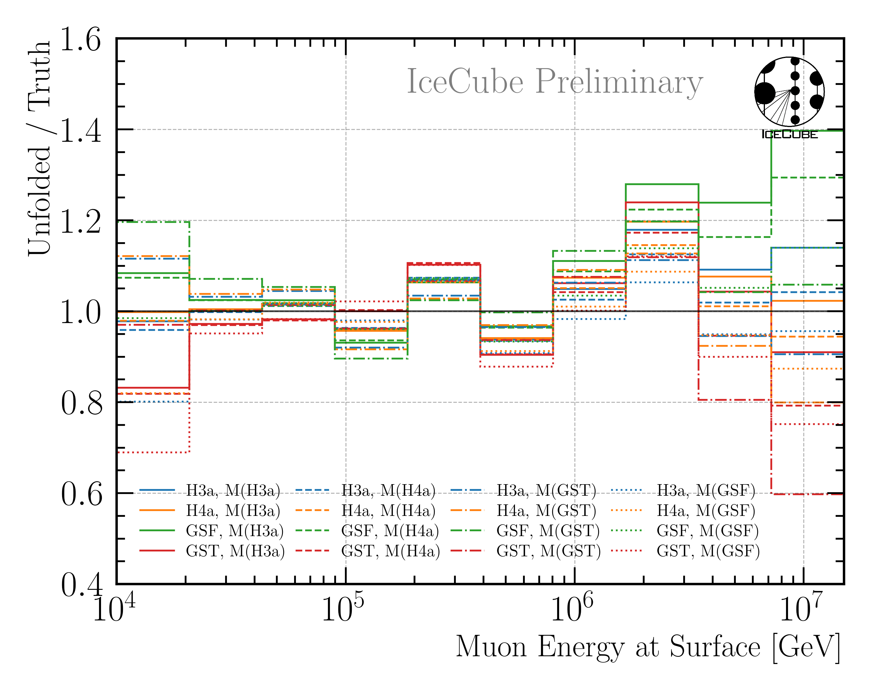
Fig. 8 : Study of the unfolding bias for the full sample unfolding. The unfolding algorithm is trained on the four different primary models, and then the MC dataset weighted to a livetime of 12 years is unfolded. The ratio to the true MC distribution is shown. This is done for all 4 weightings, which then results in 16 unfoldings in total. Ideally, all lines would align with 1. However, some deviations are visible, which are considered as unfolding bias. The maximum deviation in each bin is taken as systematic uncertainty due to the unfolding bias.
After including these uncertainties, the unfolding is able to predict the true MC distribution within the uncertainties, as shown in Fig. 238.
In Sensitivity Test, a test is performed whether the unfolding is sensitive to the prompt component. In that test, a pseudo dataset with and without prompt contribution is unfolded. The test shows that the unfolding is indeed sensitive to the prompt component.
The final prediction for the full 12 years sample is presented in Fig. 9.
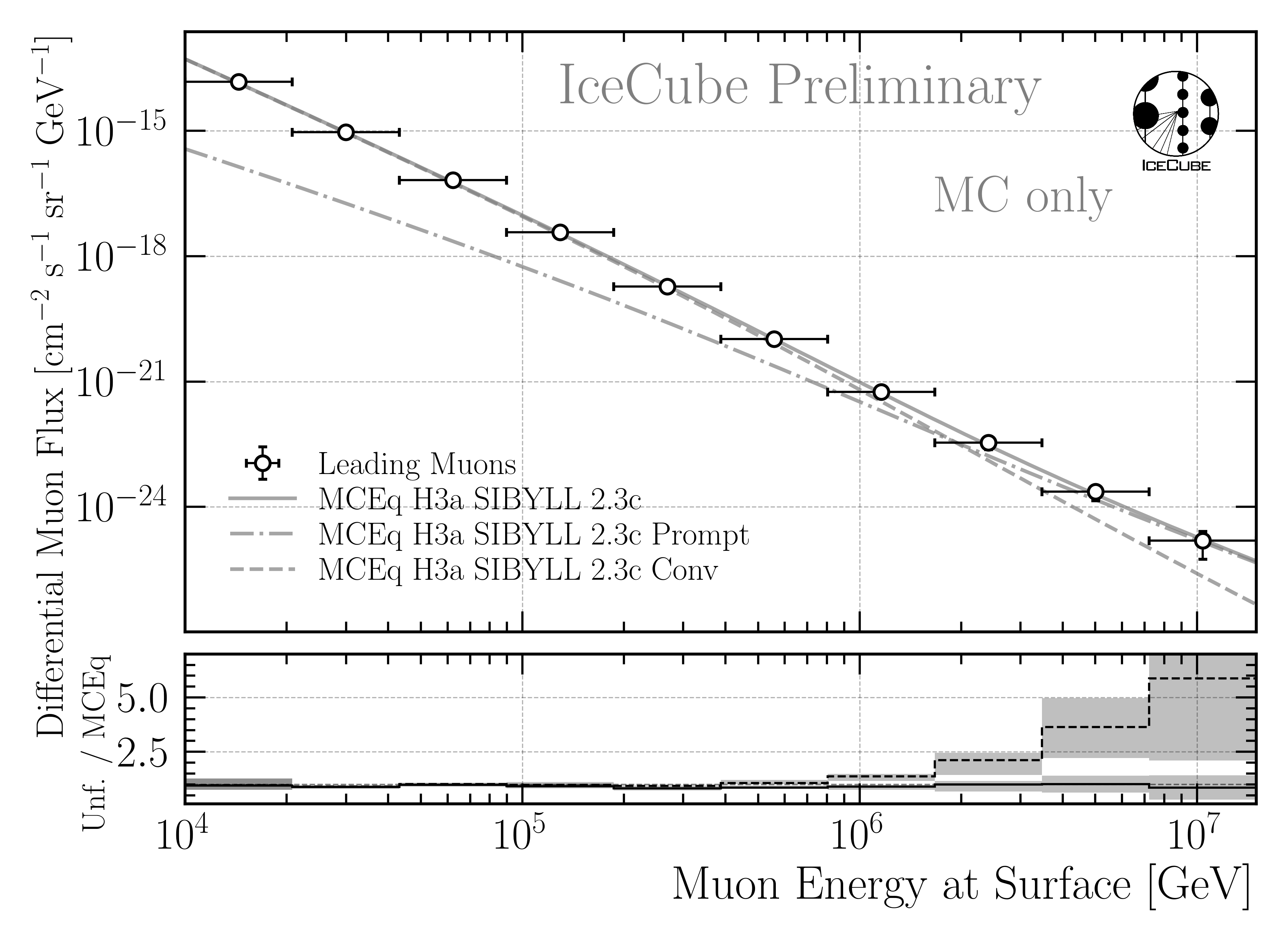
Fig. 9 : Predicted unfolded muon flux at surface for the full 12 years sample. The uncertainties are derived from the inverse of the Hessian matrix obtained in the Minuit fit and are further expanded to include the statistical uncertainties of the effective area and the unfolding bias. The unfolded result is compared to predictions from MCEq using H3a, and SIBYLL 2.3c.
The uncertainties per bin are presented in Fig. 10.
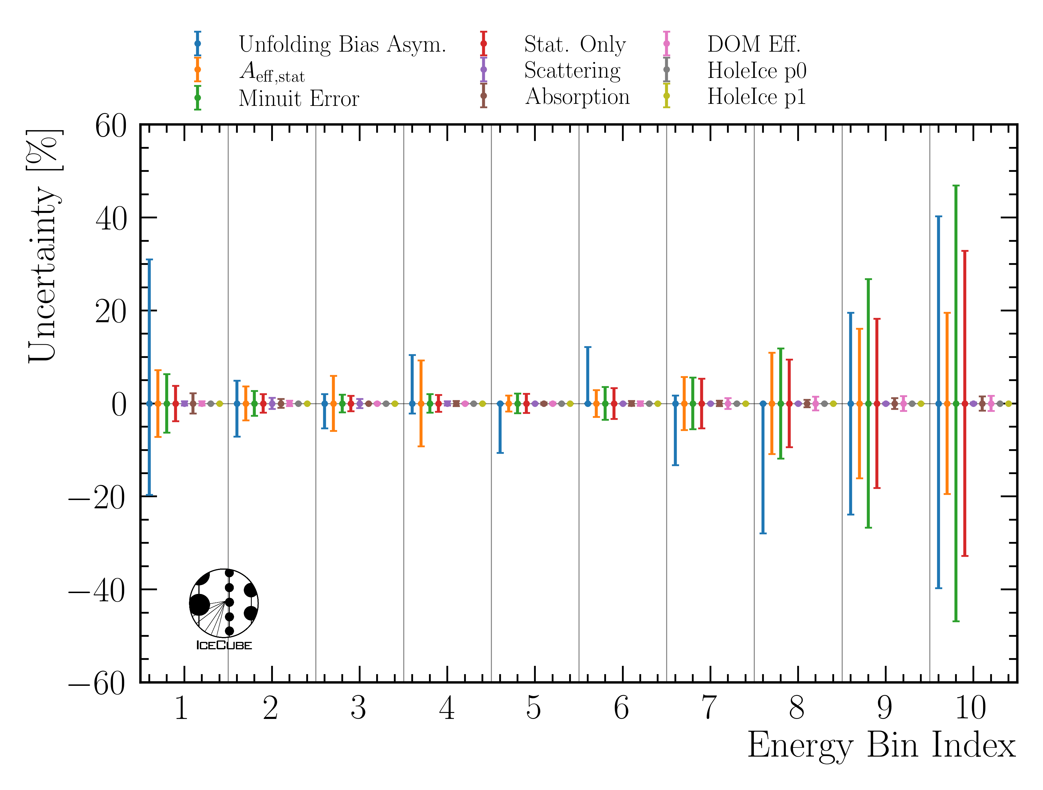
Fig. 10 : Breakdown of the different uncertainty contributions per bin for the full 12 years sample unfolding. The minuit uncertainties are derived from the inverse of the Hessian matrix obtained in the Minuit fit and are further expanded to include the 5 in-ice systematics. This is the entire minuit error. It is then divided into a statistical error and the 5 systematics each. The statistical uncertainties of the effective area and the unfolding bias are also presented.
Flux characterization (LikelihoodFitter)
The LikelihoodFitter class performs a χ²-based fit of two model components
(e.g. prompt and conventional) to measured data.
It allows for both symmetric and asymmetric per-bin uncertainties and performs
a one-sided hypothesis test for the presence of a prompt component.
Overview
Given the binned expectations for the two model components
and the measured data
the model prediction for each bin is
where \(\alpha\) and \(\beta\) are normalization parameters to be fitted.
Chi-Squared Definition
The fit minimizes the standard chi-squared function:
where \(\sigma_i\) denotes the per-bin uncertainty.
Fit Procedure
Minimization is performed with the
L-BFGS-Balgorithm, enforcing non-negative bounds for both parameters.The covariance matrix is estimated from the inverse Hessian of the fit result.
Uncertainties of the best-fit parameters are derived as:
where \(H^{-1}\) is the approximate inverse Hessian returned by the optimizer.
The fit summary reports:
\(\hat{\alpha}\), \(\hat{\beta}\) (best-fit normalizations)
\(\chi^2_\text{min}\), degrees of freedom, and \(\chi^2/\text{ndof}\)
Goodness-of-fit p-value \(p_\text{gof} = 1 - F_{\chi^2}(\chi^2_\text{min}; \text{ndof})\)
Parameter correlation from the covariance matrix
Hypothesis Test for Prompt Component
A one-sided hypothesis test evaluates whether the prompt component is required:
Null hypothesis (H₀): \(\alpha = 0\)
Alternative hypothesis (H₁): \(\alpha > 0\)
The test statistic is defined as:
and follows a ½ χ²(1) distribution (Chernoff 1954) due to the boundary at zero.
The corresponding one-sided p-value is:
which is converted into a Gaussian-equivalent significance:
Interpretation:
A small \(p\) (e.g. < 0.05) indicates evidence for a non-zero prompt component.
The reported \(Z\) value corresponds to the one-sided Gaussian significance.
Usage Example
lf = LikelihoodFitter(prompt_expectation, conv_expectation, measurement, uncertainty)

# Perform best-fit
fit_result = lf.fit()

# Perform hypothesis test for prompt component
test_result = lf.hypothesis_test()

# Print summary to console
lf.summary()
Fit prediction
Assuming symmetric unfolding bias uncertainties, the minuit uncertainties and the statistical uncertainties on the effective area, the result for a fit on MC using H3a weighting and comparing it to the CORSIKA truth is shown in Fig. 11.
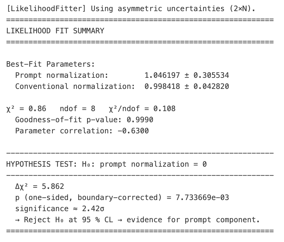
Fig. 11 : Fit of the LikelihoodFitter on MC using H3a weighting and comparing it to the CORSIKA truth. Here, symmetric uncertainties are assumed for the unfolding bias. The minuit uncertainties and the statistical uncertainties on the effective area are included. The fit is able to recover the true prompt normalization within uncertainties.